I fit a ninth-degree polynomial to eleven data points last week, purely to see what would happen. The curve threaded through every single point, and the R-squared on the fit came back as 1. Not close to one. Exactly one. I knew going in that this was going to end badly, that was the point of the exercise, but watching a model reproduce eleven numbers with that kind of confidence made something I had only understood abstractly click into place. A model that fits its training data perfectly has not necessarily learned anything about the process that generated the data. It may have simply memorised the noise.
That distinction, between fitting the data and learning the underlying pattern, is the whole game in predictive modelling, and the formal name for it is the bias-variance tradeoff.
The two ways a model can be wrong
Bias is error from a model that is too simple to capture the real relationship. Fit a straight line to a curved relationship and no amount of additional data will fix it. The line is structurally incapable of bending the way the truth bends, so it will be systematically wrong in the same direction across most of the input range. High bias models underfit. They are wrong in a stable, predictable way.
Variance is a different failure mode entirely. A model with high variance is not structurally limited, it is too sensitive. Change the training sample slightly, swap out a handful of rows, and the fitted model changes a lot. My ninth-degree polynomial on eleven points is the extreme case of this. Add one more data point, or perturb an existing one by a small amount, and the entire curve reshapes itself to accommodate it, because the model has enough free parameters to chase every wiggle in the data rather than the signal underneath it.
The tradeoff is that reducing one of these tends to increase the other. A simpler model has lower variance (it will not swing wildly from one training sample to the next) but higher bias (it cannot represent complex relationships even given unlimited data). A more flexible model can reduce bias by fitting more of the true structure, but it does so by increasing variance, because flexibility that captures real signal also captures noise it should be ignoring.
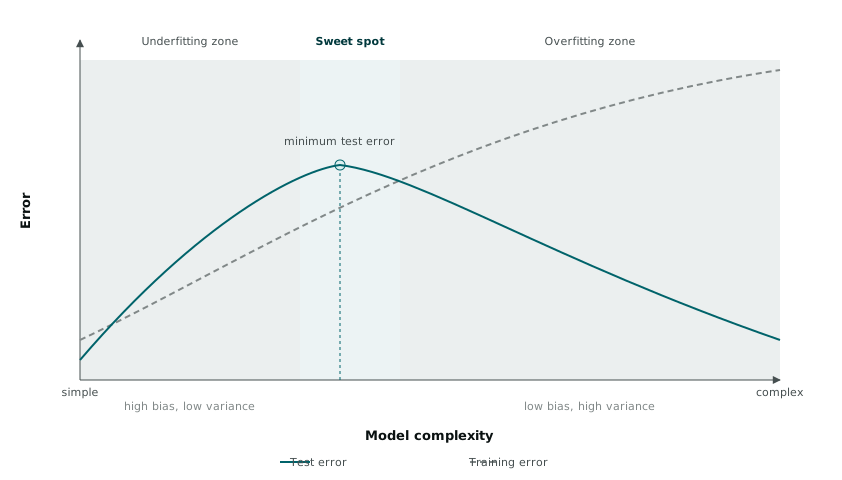
The total error a model makes on new data decomposes into these two sources plus an irreducible term from noise in the data itself that no model can remove. What that diagram is showing is the practical consequence: there is a point of model complexity where the sum of bias and variance is minimised, and it sits somewhere in the middle, not at either extreme.
Watching it happen with polynomials in R
The cleanest way I found to build intuition for this was to generate data from a known function, add noise, then fit polynomials of increasing degree and watch what happens to both training error and error on a held-out set.
set.seed(42)
n <- 40
x <- runif(n, -3, 3)
y_true <- x^3 - 4 * x^2 + 2 * x + 5
y <- y_true + rnorm(n, sd = 8)

train_idx <- sample(1:n, 28)
train_x <- x[train_idx]; train_y <- y[train_idx]
test_x <- x[-train_idx]; test_y <- y[-train_idx]

degrees <- 1:9
train_mse <- numeric(length(degrees))
test_mse <- numeric(length(degrees))

for (d in degrees) {
  fit <- lm(train_y ~ poly(train_x, d))
  train_pred <- predict(fit)
  test_pred <- predict(fit, newdata = data.frame(train_x = test_x))
  train_mse[d] <- mean((train_y - train_pred)^2)
  test_mse[d] <- mean((test_y - test_pred)^2)
}
poly(train_x, d) builds orthogonal polynomial terms up to degree d, which keeps lm() numerically stable even at higher degrees where raw powers of x would become badly correlated with each other. Plotting train_mse and test_mse against degrees reproduces the shape from the diagram almost exactly on this data. Training error falls the entire way from degree one to degree nine, because a ninth-degree polynomial has enough flexibility to bend towards every point in the training set regardless of whether that bend reflects real structure. Test error falls for the first few degrees, as the model picks up the genuine cubic shape underneath the noise, then turns and climbs back up once the extra flexibility starts fitting noise specific to the training sample rather than the underlying function.
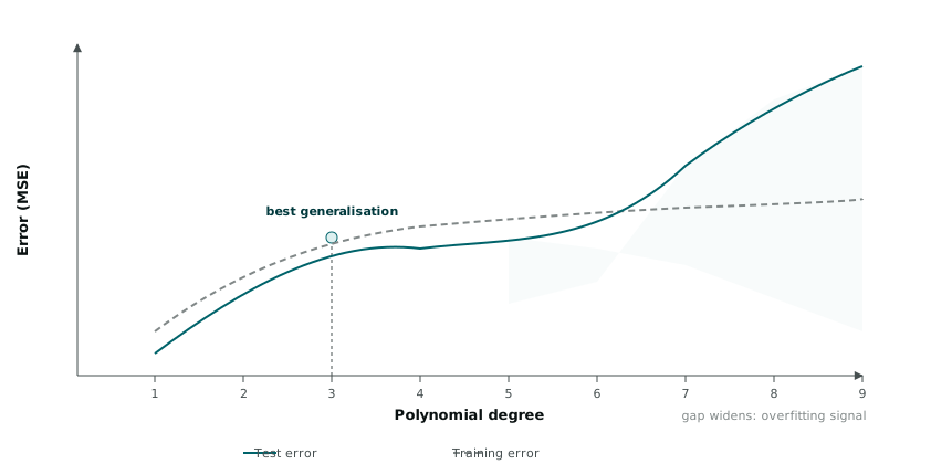
The widening gap between the two curves past the minimum is the signal to watch for, more than the absolute value of either curve. A model that fits the training data almost perfectly while doing markedly worse on held-out data is not a model that has found more structure. It has started memorising.
Why one train-test split is not enough
There is an obvious problem with the code above. I picked one random split into 28 training rows and 12 test rows, and the “best” degree that split produces depends partly on which rows landed in which set by chance. A different set.seed() value could easily shift the apparent optimum by a degree or two, particularly with a dataset this small. Making a model selection decision, choosing which degree to ship, off a single lucky or unlucky split is not a decision I want to trust.
k-fold cross-validation addresses this by rotating which rows serve as the held-out set, so every row gets used for validation exactly once and the resulting error estimate reflects an average over several different splits rather than one.
k <- 5
folds <- sample(rep(1:k, length.out = n))
cv_mse <- matrix(NA, nrow = k, ncol = length(degrees))

for (fold in 1:k) {
  fold_train_x <- x[folds != fold]; fold_train_y <- y[folds != fold]
  fold_test_x <- x[folds == fold]; fold_test_y <- y[folds == fold]

  for (d in degrees) {
    fit <- lm(fold_train_y ~ poly(fold_train_x, d))
    pred <- predict(fit, newdata = data.frame(fold_train_x = fold_test_x))
    cv_mse[fold, d] <- mean((fold_test_y - pred)^2)
  }
}

mean_cv_mse <- colMeans(cv_mse)
best_degree <- degrees[which.min(mean_cv_mse)]
sample(rep(1:k, length.out = n)) assigns each row to one of five folds in random order, so each fold gets close to an even share of the data. The outer loop rotates which fold is held out; the inner loop fits every candidate degree against whichever 32 rows are currently the training set for that fold. Averaging the five error estimates for each degree, rather than trusting any one of them, gives a far steadier read on which degree actually generalises, and best_degree came back as 3 on my synthetic data, which happens to match the true cubic relationship I generated the data from. That will not always line up so neatly on real data, where you do not get to know the ground truth in advance, but it is a satisfying check that the method is doing what it claims to.
What I take from this into real modelling work
The instinct to keep adding predictors or increasing model complexity until training error looks impressive is strong, and it is exactly the wrong instinct. Training error can only go down as you add flexibility, by construction, so it tells you almost nothing about whether the model will hold up on data it has not seen. Held-out error, ideally averaged across several folds rather than one split, is the number that matters, and the point where it stops improving and starts getting worse is the point past which you are no longer modelling the data. You are describing it.
That reframing changed how I read every model summary I have looked at since. An R-squared close to one is not automatically good news. Sometimes it is the first sign that a model has stopped being a model.