I tried to load a sensor archive into pandas and my laptop fan spun up like it was about to take off. Eight gigabytes of RAM, a CSV file sitting at eleven gigabytes on disk, and pd.read_csv() doing exactly what it is supposed to do: pull the whole thing into memory as a DataFrame before I get to run a single line of analysis on it.
It did not finish. The process sat there for four minutes, swapped memory to disk, and I killed it before it took the rest of the system down with it.
That was the moment I stopped thinking about this as a “my computer is slow” problem and started thinking about it as a “this does not fit” problem. Those are different problems with different solutions, and confusing them wastes a lot of time.
The instinct to reach for a bigger machine
The first fix I considered was the obvious one: more RAM. Rent a cloud instance with 64GB, load the file, do the work, shut it down. That works, right up until the file is 500GB, or the dataset grows past whatever RAM ceiling is economically sensible, or the analysis needs to run daily against data that keeps accumulating.
A bigger machine buys you time. It does not solve the underlying shape of the problem, which is that data volume grows faster and cheaper than single-machine memory does. Sensor networks are a clean example. A fire-detection network with a few hundred sensors, each reporting temperature, humidity, and smoke readings every sixty seconds, produces tens of millions of rows a month. Add a few years of history and the archive stops being something any one machine holds comfortably, no matter how much you spend on it.
The real fix is not a bigger machine. It is accepting that the work has to be split.
Why a single process cannot keep up
Two separate constraints show up once data grows past a certain point, and it helps to name them separately because they get fixed differently.
Memory. A pandas DataFrame lives in RAM. If the file does not fit in RAM, you cannot build the DataFrame, full stop. read_csv() has a chunksize argument that streams the file in pieces, which avoids the crash, but it does not avoid the second constraint.
CPU time. Even when a file does fit in memory, a single Python process runs on a single core by default. The Global Interpreter Lock means a stock CPython process, threading included, cannot use more than one core for CPU-bound work like parsing, aggregating, or scoring rows. Sorting fifty million rows on one core takes however long it takes. The other seven cores on your machine sit idle the entire time.
Splitting the data across partitions, and processing those partitions on separate processes, addresses both. Each process only needs enough memory for its slice. And each process runs on its own core, so the wall-clock time drops roughly in proportion to how many processes are working at once, minus whatever overhead the splitting and recombining costs.
Splitting the data: three ways to partition
Once you accept the data needs to be split, the next question is how. I tested three approaches against a sensor CSV (station id, timestamp, temperature, humidity, wind speed) to get a feel for the trade-offs before picking one for anything real.
Range partitioning. Sort by a key, usually a timestamp or an ordinal id, then split at fixed boundaries. Partition 1 gets rows with station_id 1 to 100, partition 2 gets 101 to 200, and so on. This preserves ordering within a partition, which matters if downstream code needs range queries (“all readings for stations 1 to 100”). The risk is skew. Bushfire sensor deployments cluster around known-risk regions, so a range partition by station id can leave one partition with triple the rows of another, and the whole job runs only as fast as its slowest partition.
Hash partitioning. Apply a hash function to the key and take the result modulo the number of partitions: hash(station_id) % n_partitions. This spreads rows evenly regardless of how the keys are distributed, because a good hash function does not care that stations 40 to 60 happen to be clustered in one district. The cost is that ordering is gone. Rows with adjacent station ids can land in completely different partitions, so anything that benefits from key locality (like a range scan) no longer benefits from it.
Round-robin partitioning. Assign row 1 to partition 1, row 2 to partition 2, row 3 to partition 3, and cycle back. It is the simplest scheme to implement and gives close to perfect balance for a stream of arriving rows. It throws away all key locality entirely. There is no relationship between a row’s key and the partition it ends up in, so if the next step needs “all rows for this station” grouped together, round-robin guarantees another shuffle before that is possible.
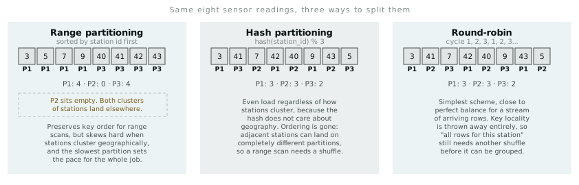
None of the three is universally correct. I ended up using hash partitioning for the sensor archive because the downstream work was per-station aggregation and I cared more about even load than about ordering. A time-series job that needed sequential windows would have pushed me toward range partitioning instead, skew and all.
Doing it with multiprocessing
Python’s multiprocessing module gives you a Pool of worker processes and a map function that hands each worker a chunk of work. For a hash-partitioned job over the sensor file, the shape looks like this:
import pandas as pd
from multiprocessing import Pool

N_PARTITIONS = 4

def partition_key(station_id):
    return hash(station_id) % N_PARTITIONS

def process_partition(df_chunk):
    return df_chunk.groupby("station_id").agg({
        "temperature": "mean",
        "humidity": "mean",
        "wind_speed": "max",
    })

df = pd.read_csv("sensor_archive.csv")
df["partition"] = df["station_id"].apply(partition_key)
partitions = [df[df["partition"] == i].drop(columns="partition")
              for i in range(N_PARTITIONS)]

with Pool(processes=N_PARTITIONS) as pool:
    results = pool.map(process_partition, partitions)

final = pd.concat(results)
Each worker gets its own partition, does the aggregation independently, and the results get concatenated at the end. Note that pool.map pickles each partition and sends it to a worker process. That serialisation is not free, and for small partitions the overhead can outweigh the benefit of parallelising in the first place. I found the break-even point on my machine sat somewhere around a few hundred thousand rows per partition. Below that, four processes ran slower than one, purely from the pickling and process-spawn cost.
Parallel is not automatically faster
The naive expectation is that four processes make a job four times faster. It rarely does, and the gap between expectation and reality comes from two places.
First, overhead. Spawning processes, pickling data across process boundaries, and merging results at the end all cost time that a single sequential run does not pay. Second, and more fundamentally, some portion of most jobs cannot be parallelised at all. Reading the source file is (usually) sequential. Concatenating the final results is sequential. Amdahl’s law formalises this: if a fixed fraction of the work is inherently serial, that fraction puts a hard ceiling on how much speedup you can ever get, no matter how many processes you throw at the parallel portion.
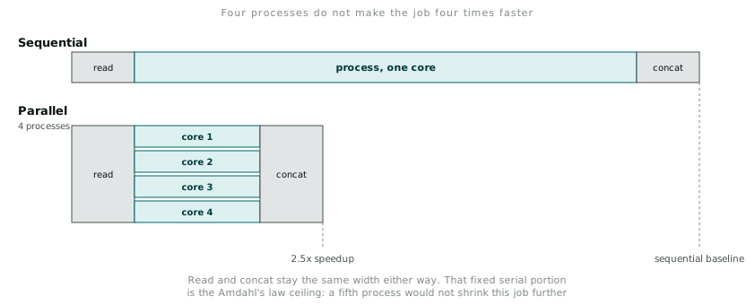
In practice this meant I stopped chasing “more cores” past four for that sensor job. The read and concat steps stayed fixed regardless of how many workers processed the middle, so beyond four processes the extra parallel capacity had nothing proportional left to speed up. Knowing where the serial floor sits mattered more than knowing how many cores the machine had.
The bigger shift was not technical, it was how I approached a dataset before writing any code. Instead of asking “how do I make this run faster on this machine,” the first question became “does this fit on this machine at all, and if not, how do I split it so each piece does.” That question changes what you build next, and it is the one that eventually leads to tools like Spark, which exist specifically to manage partitioning and scheduling for you once doing it by hand with multiprocessing.Pool stops being practical.