The feedforward network I trained on MNIST last month worked well enough, close to 98 percent accuracy on the test set, but it bothered me the moment I actually thought about what reshape(60000, 784) was doing to the data going in. Flattening a 28 by 28 image into a single row of 784 numbers throws away every piece of spatial information the image had. Pixel 27 and pixel 55 sit right next to each other in the original grid, one row apart, but once flattened they are just two entries in a long vector with no indication that they were ever neighbours. The network has to relearn spatial relationships from scratch, purely from statistical patterns in the training data, when that relationship was sitting right there in the raw pixels the whole time.
Convolutional layers exist to stop throwing that information away. Instead of treating an image as a flat list of independent numbers, a convolutional layer treats it as a grid and applies the same small operation, a filter, across every local neighbourhood of that grid. Two assumptions make this work, and once I saw them named separately it became obvious why CNNs do so much better on image data. The first is locality, that a pixel’s meaning depends mostly on its nearby neighbours, an edge or a curve is a local pattern, not something that depends on comparing opposite corners of the image. The second is translation invariance, that a useful pattern, a diagonal edge, a loop, a corner, is worth detecting the same way regardless of where in the image it happens to appear. A dense layer has to learn a separate weight for every single pixel position. A convolutional layer learns one small filter and reuses it everywhere.
What a convolution actually does
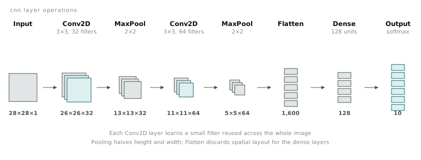
A filter, also called a kernel, is a small matrix of weights, commonly 3x3 for the kind of network I have been building. The layer slides that 3x3 window across the input image, and at every position it computes a weighted sum of the pixels underneath it, producing one output value per position. Slide the whole window across the entire image and the result is a new grid, smaller than the original, called a feature map. A convolutional layer with 32 filters is not learning one pattern detector, it is learning 32 of them in parallel, each producing its own feature map, so a single Conv2D layer on a 28x28 greyscale input produces 32 separate feature maps of roughly the same spatial size.
from keras.models import Sequential
from keras.layers import Conv2D, MaxPooling2D, Flatten, Dense

model = Sequential()
model.add(Conv2D(32, kernel_size=(3, 3), activation='relu', input_shape=(28, 28, 1)))
model.add(MaxPooling2D(pool_size=(2, 2)))
model.add(Conv2D(64, kernel_size=(3, 3), activation='relu'))
model.add(MaxPooling2D(pool_size=(2, 2)))
model.add(Flatten())
model.add(Dense(128, activation='relu'))
model.add(Dense(10, activation='softmax'))
The input shape here is (28, 28, 1) rather than the flattened (784,) from my dense network, because Conv2D expects height, width, and channel count, one channel for greyscale, three if this were colour. That meant reshaping the MNIST arrays differently at the loading stage.
x_train = x_train.reshape(60000, 28, 28, 1).astype('float32') / 255
x_test = x_test.reshape(10000, 28, 28, 1).astype('float32') / 255
MaxPooling2D downsamples each feature map by taking the maximum value in every 2x2 block, halving both height and width. It is doing two jobs at once. It reduces the amount of computation needed in every layer after it, and it makes the network somewhat more tolerant of small shifts in exactly where a feature sits, since the max over a 2x2 region does not change if the strongest activation moves by a pixel within that region. Flatten at the end converts the final stack of small feature maps back into a single vector, which is the point where the network stops caring about spatial layout and hands off to ordinary dense layers for the classification decision.
Where the parameter count goes
The thing that convinced me convolutions were not just a fashionable alternative to dense layers was looking at what model.summary() reports for parameter counts.
model.summary()Layer (type) Output Shape Param #
=================================================================
conv2d_1 (Conv2D) (None, 26, 26, 32) 320
max_pooling2d_1 (MaxPooling2 (None, 13, 13, 32) 0
conv2d_2 (Conv2D) (None, 11, 11, 64) 18496
max_pooling2d_2 (MaxPooling2 (None, 5, 5, 64) 0
flatten_1 (Flatten) (None, 1600) 0
dense_1 (Dense) (None, 128) 204928
dense_2 (Dense) (None, 10) 1290
=================================================================
Total params: 225,034The first Conv2D layer has 320 parameters. That number comes from a 3x3 filter, 9 weights, times 32 filters, plus one bias per filter, (3 * 3 * 1 + 1) * 32 = 320. Compare that with the first dense layer in my feedforward network from last month, which connected 784 flattened inputs to 128 hidden units, 784 * 128 + 128 = 100,480 parameters, in that single layer alone. The convolutional layer produces 32 entire feature maps covering the whole image and does it with roughly three hundred times fewer parameters than one dense layer needed just to look at the raw pixels once.
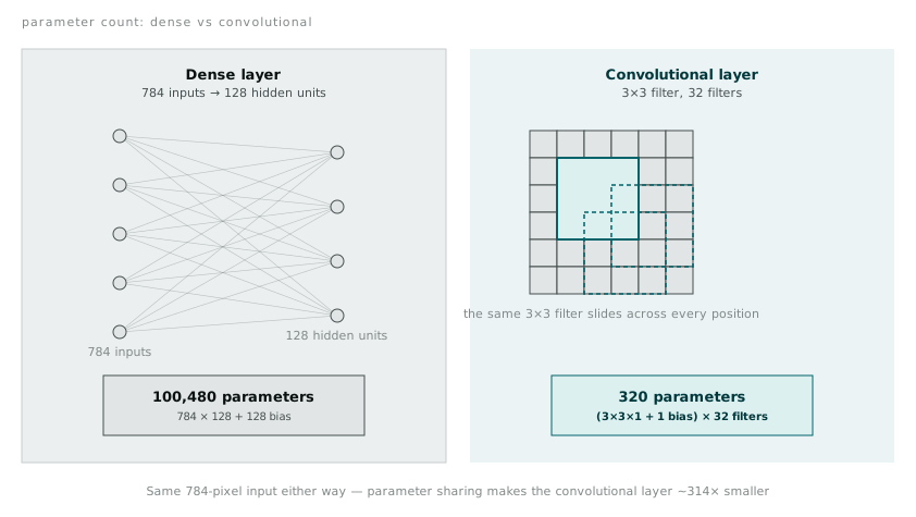
That gap is parameter sharing, the same 3x3 filter weights get reused at every single position as the window slides across the image, rather than each position getting its own independent set of weights the way a dense layer’s connections work. A dense layer effectively learns a separate detector for “is there a vertical edge in the top left corner” and a completely unrelated detector for “is there a vertical edge in the bottom right corner.” A convolutional filter learns one vertical edge detector and applies it everywhere, which matches the translation invariance assumption exactly and means far less has to be learned from the training data before the filter generalises.
Comparing accuracy against the dense network
I trained both architectures on the same MNIST split, same 10 epochs, same batch size of 32, to see whether the parameter efficiency actually translated into anything measurable rather than just being architecturally elegant.
model.compile(optimizer='adam', loss='categorical_crossentropy', metrics=['accuracy'])
history = model.fit(x_train, y_train, epochs=10, batch_size=32, validation_split=0.1)
test_loss, test_accuracy = model.evaluate(x_test, y_test)
print(f'CNN test accuracy: {test_accuracy:.4f}')
The CNN came out around 0.989 on the test set, against 0.976 for the dense network from before. A little over one percentage point sounds small written down, but on MNIST, a dataset every architecture already does reasonably well on, that gap represents a meaningful chunk of the remaining error being eliminated. I ran the same comparison on Fashion-MNIST, the clothing item dataset built as a drop in replacement for MNIST once people noticed digit classification had become too easy to distinguish good architectures from mediocre ones, and the gap widened considerably there, the dense network struggling into the mid eighties while the CNN pushed past ninety. Clothing items apparently have more spatial structure worth exploiting than handwritten digits do, sleeves and collars and hems occurring in roughly consistent relative positions, which the convolutional layers pick up on and the flattened dense network cannot.
The trade-off I am not sure about yet
None of this is free. Training the CNN took noticeably longer per epoch than the dense network did, even though it has fewer total parameters, because sliding a filter across an entire image involves a lot more individual multiply-add operations than a single dense matrix multiplication covering the same input. Fewer parameters does not mean fewer computations, and I had assumed those two things tracked each other more closely than they do. I also have not yet worked out how deep is reasonable to go, whether stacking three or four Conv2D and MaxPooling2D pairs instead of two would keep improving accuracy or start overfitting on a dataset this size, and whether the answer changes once the images stop being 28x28 greyscale digits and become something with real texture and colour. That feels like the next thing worth testing rather than reading about.