My First Neural Network with TensorFlow and Keras

I spent an evening a few weeks back playing with TensorFlow Playground, the browser demo where you drag sliders and watch a tiny neural network carve up a scatter of orange and blue dots. It is a toy, deliberately so, but watching the decision boundary bend and twist as I added layers and changed activation functions did something none of my reading on backpropagation had managed. It made the whole thing feel mechanical rather than mysterious. I understood gradient descent well enough on paper, the chain rule pushing an error signal backwards through a stack of weights. I had never actually trained a network. So I installed TensorFlow and Keras on my own machine and set out to close that gap.

The install itself was the first surprise, mostly because Keras and TensorFlow are two separate packages that happen to work together rather than one library.

pip install tensorflow
pip install keras

TensorFlow is the computational engine. It builds a graph of operations, hands that graph to a session, and runs data through it via placeholders and a feed_dict, all of which is fairly unforgiving if you try to work with it directly. Keras sits on top as a higher-level API and hides almost all of that scaffolding behind a much friendlier interface. I did not end up touching a tf.Session directly for this first attempt, which was the entire point of starting with Keras rather than raw TensorFlow.

MNIST, because everyone starts here

MNIST is the handwritten digit dataset, seventy thousand small greyscale images of digits zero through nine, twenty eight pixels square. It ships with Keras as a convenience loader, which meant I skipped the usual data wrangling step and went straight to looking at what I was working with.

from keras.datasets import mnist

(x_train, y_train), (x_test, y_test) = mnist.load_data()

print(x_train.shape)  # (60000, 28, 28)
print(y_train.shape)  # (60000,)

Sixty thousand training images, ten thousand held out for testing, each one a 28 by 28 array of pixel intensities from 0 to 255. The labels are single integers, 0 through 9, telling you which digit each image shows. Before any of that goes into a network I flattened each image into a single vector of 784 values and scaled the pixel intensities down to the 0 to 1 range, because gradient descent behaves far better with inputs on a small, consistent scale than with raw pixel values in the hundreds.

x_train = x_train.reshape(60000, 784).astype('float32') / 255
x_test = x_test.reshape(10000, 784).astype('float32') / 255

The labels need one more transformation. A raw integer like 7 does not mean anything to a network trained with a softmax output and categorical cross entropy loss, since the loss function expects a probability distribution to compare against, not a single number. Keras has a utility for this.

from keras.utils import to_categorical

y_train = to_categorical(y_train, 10)
y_test = to_categorical(y_test, 10)

to_categorical turns the integer 7 into a ten element vector, all zeros except for a 1 in position seven. One hot encoding, in other words, which I had already used plenty of times on categorical predictors in regression work. Seeing it show up here, doing the same job for a different reason, was a small but useful bit of a pattern repeating across two fields I had been treating as separate.

Building the network

Keras has two ways to define a model, a functional API for anything with branches or multiple inputs, and the Sequential model for the plain case where data flows through one layer after another with no forks. A feedforward classifier on flattened pixel data is exactly that plain case.

from keras.models import Sequential
from keras.layers import Dense

model = Sequential()
model.add(Dense(128, activation='relu', input_shape=(784,)))
model.add(Dense(64, activation='relu'))
model.add(Dense(10, activation='softmax'))

Three lines, three layers, and each one is doing something specific enough that it was worth slowing down on. The first Dense(128) takes the 784 pixel values and maps them onto 128 units, each one a weighted sum of all 784 inputs plus a bias, passed through a ReLU activation. ReLU is just max(0, x), which sounds too simple to matter, but it is what lets stacking layers actually add expressive power rather than collapsing into one big linear function, since a stack of purely linear layers is mathematically equivalent to a single linear layer no matter how many you chain together. The second Dense(64) does the same thing again on a smaller scale, taking the 128 outputs from the first layer down to 64. The last layer maps down to 10 units, one per digit, with a softmax activation that turns the raw outputs into a probability distribution across the ten classes, all positive and summing to one.

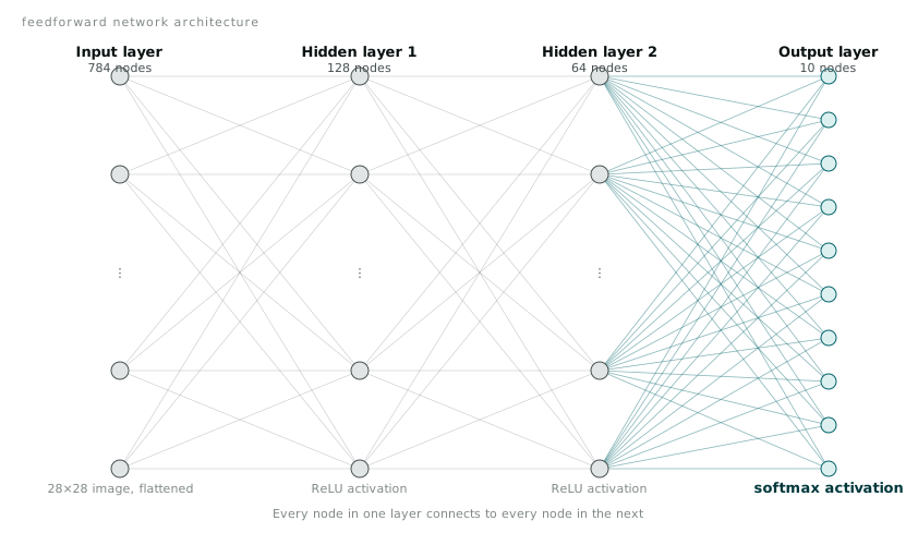
None of the numbers here, 128 and 64 in particular, came from a formula. They are common starting points, powers of two mostly out of habit from how GPUs handle memory, and I picked them because they were what most introductory examples used rather than because I had a principled reason to prefer them over 100 and 50. That is worth being honest about. A fair amount of network architecture at this stage of learning is inherited convention rather than derivation.

Compiling: choosing how the network learns

Building the layers only defines the shape of the network. Before it can learn anything I have to tell Keras three more things, how to measure error, how to adjust weights in response to that error, and what to report while training.

model.compile(
    optimizer='adam',
    loss='categorical_crossentropy',
    metrics=['accuracy']
)

categorical_crossentropy is the loss function, and it is the natural pairing for a softmax output and one hot encoded labels, penalising the network heavily when it assigns low probability to the correct class. adam is the optimiser, a variant of gradient descent that adapts its own learning rate per parameter as training proceeds rather than using one fixed step size for every weight in the network. I had read the Adam paper’s abstract without really absorbing what “adaptive moment estimation” meant in practice. Using it here without having derived it myself felt like a small compromise, trusting a well-established default rather than working through the maths first, but the maths behind Adam involves tracking running averages of both the gradient and the squared gradient, moment estimates in the paper’s terms, and I decided that understanding what it does for training stability mattered more right now than re-deriving why it works.

Fitting and evaluating

With the model compiled, training is one call.

history = model.fit(
    x_train, y_train,
    epochs=10,
    batch_size=32,
    validation_split=0.1
)

An epoch is one full pass through the training data. Batch size of 32 means the network looks at 32 images, computes the average loss across them, and updates its weights once, rather than updating after every single image or waiting until it has seen all sixty thousand. validation_split=0.1 holds back ten percent of the training set to check the model against after each epoch, giving a running sense of whether it is generalising or just memorising the training examples. Watching the printed output scroll past for ten epochs, training loss falling steadily while validation accuracy climbed into the high nineties, was the single most satisfying part of the whole exercise. Something I had built from three lines of layer definitions was demonstrably learning to recognise handwriting.

test_loss, test_accuracy = model.evaluate(x_test, y_test)
print(f'Test accuracy: {test_accuracy:.4f}')

evaluate runs the trained model against the held out test set, images it never saw during training in any form, not even the validation split, and returns the same loss and accuracy figures. Mine came out around 0.976, which is well short of state of the art on MNIST but respectable for a first network with no tuning applied.

What Keras is quietly doing for you

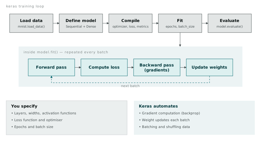
The part that took the longest to sit right with me is how much fit() is doing behind that one function call. Under the hood, each batch triggers a forward pass through the network, a loss calculation, a backward pass computing the gradient of that loss with respect to every weight via backpropagation, and a weight update from the optimiser, all running inside a TensorFlow session with placeholders feeding data in and a graph of operations executing the actual maths. None of that is visible from the Keras side. I know the theory well enough to have written a two layer network’s backpropagation by hand on paper before, gradients and all, which is exactly why the abstraction here felt earned rather than like cheating. I was not skipping understanding what happens underneath. I was choosing not to reimplement it, because Keras implementing it correctly and efficiently is the entire reason it exists.

What I do still specify, and what actually matters for getting a working model, is the architecture, how many layers and how wide, the activation functions, the loss and optimiser, and the training schedule, epochs and batch size. Those choices are where the judgement lives. Everything Keras automates is the mechanical part that would be identical regardless of which specific network I was training. That divide, between decisions that require understanding the problem and computation that is the same every time, is roughly where I now think the actual skill in this area sits, at least for the kind of standard architectures I am starting with.

I have not touched convolutional layers yet, which feel like the obvious next step given that flattening a 28 by 28 image into 784 independent numbers throws away all the spatial structure in it, the fact that a pixel’s neighbours tend to matter more than a pixel on the opposite corner of the image. That is a problem for another evening.