I have called lm() in R more times than I could count, and for most of that time I treated the fitting step as a black box that took a formula and a data frame and handed back coefficients. That was fine for ordinary least squares, which has a closed-form solution and does not need iteration at all. It stopped being fine the moment I looked at a logistic regression cost function and realised there is no equivalent closed form, and the thing quietly doing the work underneath almost every model that cannot be solved analytically is gradient descent. I wanted to understand that loop well enough to trust it, not just invoke it.
The problem gradient descent solves
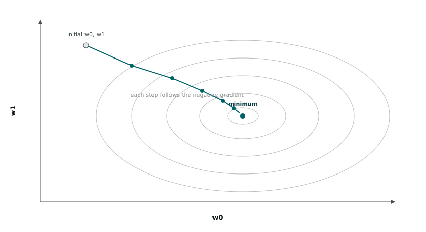
Fitting a linear model means choosing an intercept and a slope, call them w0 and w1, that minimise the sum of squared errors between predictions and actual values. For simple linear regression this has a direct algebraic answer, the normal equations, and R computes it that way under the hood. But the cost surface for that problem, plotted against w0 and w1, is a smooth bowl shape, convex, with exactly one minimum. Gradient descent is a general method for finding the bottom of a bowl like that (or something close to it, for surfaces that are not so cleanly convex) without solving for it algebraically. Start somewhere on the surface, work out which direction is downhill, take a step in that direction, and repeat until the steps stop moving you anywhere useful.
“Which direction is downhill” is exactly what the gradient tells you. The gradient of the cost function with respect to the parameters is a vector pointing in the direction of steepest increase, so taking a step in the opposite direction moves towards lower cost.
Deriving the update rule
For a linear model with one predictor, the prediction is y_hat_i = w0 + w1 * x_i, and the cost function, mean squared error over n training rows, is
J(w0, w1) = (1/n) * sum_i (y_i - w0 - w1 * x_i)^2Taking the partial derivative with respect to w0 and applying the chain rule:
dJ/dw0 = (-2/n) * sum_i (y_i - w0 - w1 * x_i)and with respect to w1:
dJ/dw1 = (-2/n) * sum_i (y_i - w0 - w1 * x_i) * x_iEach of those is a sum over the residuals, either raw or weighted by x_i, which is worth sitting with, because it means the gradient is entirely made of numbers you could compute with lm()’s fitted values and a couple of vector operations. The update rule takes a step of size alpha, the learning rate, against that gradient:
w0 <- w0 - alpha * dJ_dw0
w1 <- w1 - alpha * dJ_dw1
Subtracting rather than adding is the whole trick. The gradient points uphill, so moving against it moves downhill.
Batch gradient descent in R
x <- c(1, 2, 3, 4, 5, 6, 7, 8)
y <- c(2.1, 3.9, 6.2, 7.8, 10.1, 11.9, 14.2, 15.8)
n <- length(x)

w0 <- 0; w1 <- 0
alpha <- 0.01
iterations <- 1000
history <- data.frame(iter = 1:iterations, cost = NA)

for (i in 1:iterations) {
  pred <- w0 + w1 * x
  error <- y - pred

  grad_w0 <- -2 / n * sum(error)
  grad_w1 <- -2 / n * sum(error * x)

  w0 <- w0 - alpha * grad_w0
  w1 <- w1 - alpha * grad_w1

  history$cost[i] <- mean(error^2)
}

cat("w0:", round(w0, 3), " w1:", round(w1, 3), "\n")
This is called batch gradient descent because every single update uses all eight rows of x and y to compute the gradient before taking a step. On data this small it runs in a blink, and after a thousand iterations w0 and w1 land close enough to what lm(y ~ x) returns directly that the difference is a rounding error. Plotting history$cost against history$iter shows a curve that drops fast at first and flattens as it nears the minimum, which is exactly what you would expect from a step size proportional to the gradient. Big gradient early on, when far from the minimum, means big steps. Gradient shrinks to near zero close to the minimum, so steps shrink with it.
Stochastic gradient descent
Batch gradient descent needing the whole dataset for every single step is fine for eight rows and a serious constraint for anything large. Stochastic gradient descent updates the parameters using one randomly chosen row at a time instead of the full sum.
w0 <- 0; w1 <- 0
alpha <- 0.01
epochs <- 50

for (epoch in 1:epochs) {
  shuffled <- sample(1:n)
  for (i in shuffled) {
    pred_i <- w0 + w1 * x[i]
    error_i <- y[i] - pred_i

    w0 <- w0 - alpha * (-2 * error_i)
    w1 <- w1 - alpha * (-2 * error_i * x[i])
  }
}
Each pass through the shuffled data is one epoch. The per-row gradient is a noisy estimate of the true batch gradient, since it is based on a single point rather than an average across all of them, so the path SGD takes towards the minimum zigzags rather than descending smoothly. That noise is not pure downside. On far larger datasets it means every update is cheap, and the randomness can help the parameters avoid getting permanently stuck in a shallow local dip on cost surfaces that are not as clean and convex as ordinary least squares. For this eight-row example the two methods land in essentially the same place, and the only honest reason to reach for SGD here would be to see the zigzag for myself.
Getting the learning rate wrong in both directions
The learning rate (\alpha) is the one knob in this whole process, and getting it wrong breaks the algorithm in two distinct ways rather than one.
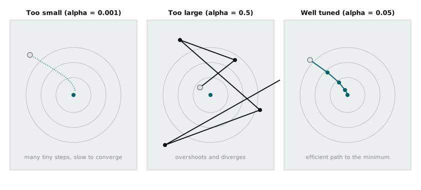
Set (\alpha) too small and every step barely moves. The algorithm will still converge eventually, given a convex surface, but “eventually” might mean waiting for tens of thousands of iterations to reach a result a properly tuned rate would have reached in a few dozen. Set (\alpha) too large and the step taken based on the current gradient overshoots the minimum entirely, landing somewhere on the far side of the bowl with a gradient pointing back the other way, at which point the next step overshoots again, larger this time because it is being computed from a point further out on the surface. On a bowl shaped cost function this pattern compounds, and the cost history that would normally fall stops falling and starts growing without bound. I reproduced this by accident the first time I tried an aggressive alpha of 0.5 on the batch loop above. history$cost went from a small number to Inf within about a dozen iterations, and watching that happen was a far more convincing lesson in the failure mode than any explanation of it would have been.
There is no single correct learning rate independent of the problem. It depends on the scale of the features and the curvature of the cost surface, which is part of why standardising predictors before fitting is common practice, it keeps the gradient magnitudes in a range where a single learning rate works reasonably across all the coefficients rather than being too aggressive for one and too timid for another.
What changed after doing this by hand
Watching the cost drop, plateau, or blow up on tiny synthetic data made the abstraction behind every .fit() call in every library I have used feel less like magic and more like a loop I could have written myself, because I had. That does not mean I plan to hand-roll gradient descent for anything beyond a learning exercise, the production implementations handle numerical edge cases and convergence checks I have not bothered with here. But knowing what is happening inside the loop changes how I read a training curve that refuses to converge. It is very often exactly this, a learning rate fighting the shape of the surface, rather than something more exotic.