The fire-detection sensor archive from a few weeks back was still sitting on my disk when I decided to do something more useful with it than aggregate temperature averages. A bushfire risk-scoring exercise, which I started calling StopFire in my notes because it needed a name and that one stuck, needed two datasets joined together: sensor readings (station id, timestamp, temperature, humidity, wind speed) and Bureau of Meteorology regional weather CSVs (station id, timestamp, rainfall, forecast fire danger rating). Same key, two files, one join.
I could have written pd.merge() and had an answer in one line. I did not, on purpose. I wanted to know what a join actually costs before I let a library do it invisibly, so I built search, join, sort, and group-by by hand using multiprocessing.Pool, over partitions I controlled myself. It took a full weekend. It also changed how I read every Spark execution plan I have looked at since.
Why bother when pandas already has merge
pd.merge() is a hash join under the hood, single-threaded, and it works fine until the data does not fit comfortably in memory or the join key is skewed enough that a single core spends most of its time on one ugly partition. Neither of those was true for my StopFire files yet. I built the parallel versions anyway because I wanted the mental model, not the speedup. Once you have written a merge sort with your own hands, “shuffle” stops being a word Spark’s UI shows you and starts being a specific, physical thing that happens to specific rows.
Parallel search: partition, scan, merge
The simplest of the four. Given a station id, find every sensor reading matching it across a 40-million-row archive split into partitions.
import pandas as pd
from multiprocessing import Pool

N_PARTITIONS = 8

def search_partition(args):
    df_chunk, target_id = args
    return df_chunk[df_chunk["station_id"] == target_id]

def parallel_search(partitions, target_id):
    with Pool(processes=N_PARTITIONS) as pool:
        results = pool.map(search_partition, [(p, target_id) for p in partitions])
    return pd.concat(results, ignore_index=True)
Each worker does a linear scan of its own partition. There is no cleverness here beyond fanning the scan out across cores and concatenating whatever comes back. For a single lookup against 40 million rows, this beat a sequential df[df.station_id == target_id] by a factor that scaled roughly with core count, minus pickling overhead for shipping each partition to its worker.
The lesson that stuck: search parallelises embarrassingly well because there is no coordination between partitions. Nothing a worker finds in partition 3 depends on what a worker finds in partition 7. Join and sort are not so forgiving.
Parallel join: the part that actually taught me something
A join needs matching rows to land in the same place before they can be compared, and two independently-partitioned datasets have no guarantee their matching rows sit in corresponding partitions. The fix is to partition both inputs by the same key using the same hash function, so that everything with station_id = 14, from either dataset, ends up in partition hash(14) % N, regardless of which file it came from.
def hash_partition(df, key_col, n_partitions):
    df = df.copy()
    df["_part"] = df[key_col].apply(lambda k: hash(k) % n_partitions)
    return [df[df["_part"] == i].drop(columns="_part") for i in range(n_partitions)]

def join_partition(args):
    sensor_chunk, weather_chunk = args
    return pd.merge(sensor_chunk, weather_chunk, on=["station_id", "timestamp"], how="inner")

def parallel_join(sensor_df, weather_df, n_partitions=8):
    sensor_parts = hash_partition(sensor_df, "station_id", n_partitions)
    weather_parts = hash_partition(weather_df, "station_id", n_partitions)
    with Pool(processes=n_partitions) as pool:
        results = pool.map(join_partition, zip(sensor_parts, weather_parts))
    return pd.concat(results, ignore_index=True)
Each worker runs a small, ordinary pd.merge() on its own matching pair of partitions. The parallel part is not the join logic itself, it is getting matching keys colocated before the join runs. That repartition step is what Spark calls a shuffle, and it is not free. Data has to move between partitions, get pickled, sent across process boundaries, and reassembled. For my sensor and weather files, roughly a third of total wall-clock time went into the two hash_partition() calls, not the actual pd.merge() calls inside each worker.
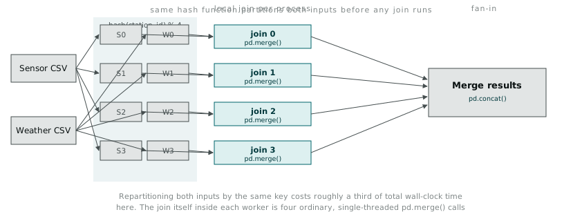
That third of the time is the price of correctness. Skip the repartition and you get a join that misses matches sitting in the wrong partition on each side, silently, with no error to tell you rows went missing.
Parallel sort: sample first, sort second
Sorting is where naive partitioning falls over completely. Sort each partition independently and concatenate, and you get eight locally-sorted chunks that are globally out of order, station 400 appearing after station 12 in the final output because it happened to land in an earlier partition.
The fix, a simplified version of sample sort, is to choose partition boundaries before sorting, not after:
import numpy as np

def choose_boundaries(df, key_col, n_partitions, sample_frac=0.01):
    sample = df[key_col].sample(frac=sample_frac).sort_values()
    quantile_points = np.linspace(0, 1, n_partitions + 1)[1:-1]
    return sample.quantile(quantile_points).tolist()

def range_partition(df, key_col, boundaries):
    return np.searchsorted(boundaries, df[key_col])

def sort_partition(df_chunk):
    return df_chunk.sort_values("timestamp")

def parallel_sort(df, key_col="timestamp", n_partitions=8):
    boundaries = choose_boundaries(df, key_col, n_partitions)
    df = df.copy()
    df["_part"] = range_partition(df, key_col, boundaries)
    parts = [df[df["_part"] == i].drop(columns="_part") for i in range(n_partitions)]
    with Pool(processes=n_partitions) as pool:
        sorted_parts = pool.map(sort_partition, parts)
    return pd.concat(sorted_parts, ignore_index=True)
Sample 1% of the data, find quantile boundaries from that sample, and use those boundaries to route every row into the partition that owns its range. Partition 0 gets everything below the first boundary, partition 1 gets everything between the first and second, and so on. Because the boundaries came from quantiles, each worker now sorts a range that is already known to sit entirely before or after every other worker’s range. Concatenate the sorted partitions in order and the whole dataset comes out globally sorted, with no final merge step needed.
The subtlety I missed on the first attempt: the sample has to be representative. I sampled too small a fraction on my first pass (0.1%) against a dataset with a lumpy timestamp distribution, weeks with far more sensor readings than others, and ended up with one partition holding four times the rows of its neighbours. The boundaries were technically correct, evenly spaced across the sampled quantiles, but the underlying data was not evenly distributed across those same quantile ranges. Bumping the sample to 1% fixed it. Below a certain sample size, you are choosing boundaries based on noise.
Parallel group-by: reduce, don’t just map
Group-by looks like search at first glance (fan out, do work per partition) until you notice a station’s readings can span multiple partitions if the data was hash-partitioned by timestamp rather than station id. The fix is the same repartition-then-local-work pattern as join: hash by the grouping key first, so every reading for a given station lands in one partition, then each worker runs its own groupby().agg() with no cross-partition coordination needed at all.
def group_partition(df_chunk):
    return df_chunk.groupby("station_id").agg({
        "temperature": "mean",
        "rainfall": "sum",
        "wind_speed": "max",
    })

def parallel_groupby(df, key_col="station_id", n_partitions=8):
    parts = hash_partition(df, key_col, n_partitions)
    with Pool(processes=n_partitions) as pool:
        results = pool.map(group_partition, parts)
    return pd.concat(results)
Because the hash partition guarantees each station’s rows are together in one place, there is no second aggregation pass needed after the workers finish, the way there would be if a station’s rows were scattered across partitions and each worker only had a partial view.
Putting it together for StopFire
The actual StopFire scoring run chained all four: hash-partition the sensor and weather files by station id, parallel-join them, parallel-search for stations above a wind speed threshold within the joined result, and parallel-group-by station to compute a rolling risk score from temperature, low humidity, and BOM fire danger rating together.
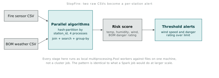
None of this is production code. There is no fault tolerance if a worker process dies partway through, no spill-to-disk when a partition does not fit in memory, and no scheduler deciding how many partitions make sense for the cluster you actually have. That is precisely the list of things Spark does for you, and until I had written the repartition-then-local-work pattern myself, three separate times, for three different operations, I did not have a real feel for why that list matters. A shuffle in a Spark stage plan is not an abstract cost anymore. It is the exact hash-partition step I wrote by hand, running on a cluster instead of eight local processes, with the same skew risk and the same repartitioning bill attached.
The other thing the exercise settled for me: multiprocessing.Pool is a fine tool for a laptop-sized dataset and a hard stop past it. Every partition here still had to fit in one worker’s memory, and I was still bound to however many cores sat in one machine. The pattern scales to a cluster. The tool in front of me that weekend did not.