Every classification model I had built up to this point started from a column of known labels. Fraud or not fraud, churned or retained, something a human had already decided and recorded. I sat down recently with a pile of short text documents that had no such column, no topic label anywhere, and the instruction was effectively “find the groups yourself.” That is a genuinely different problem, not a smaller version of the same one, and it needed a different kind of learning to solve it.
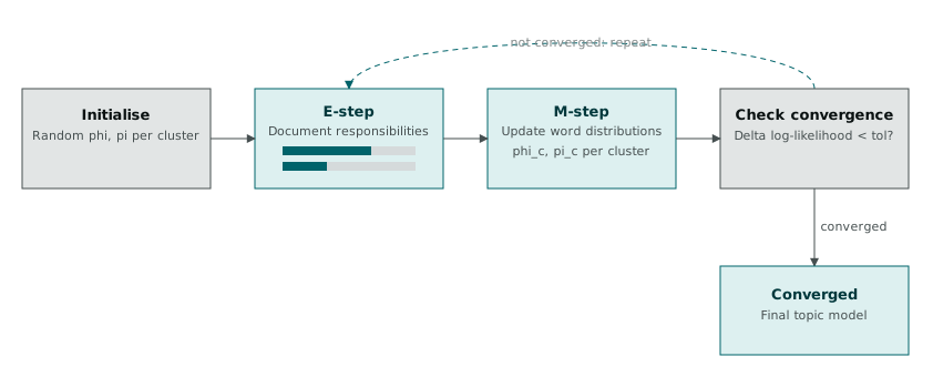
I had already worked through the EM algorithm for clustering numeric measurements into Gaussian mixture components. The same algorithm, expectation-maximisation, applies here too, with one change that matters: instead of assuming each cluster generates points from a Gaussian, each cluster generates a document by repeatedly drawing words from its own distribution over the vocabulary. Swap the distribution family and the same two-step machinery carries across.
Setting up the model
Represent each document as a vector of word counts over a fixed vocabulary, the standard bag-of-words treatment that throws away order and keeps only frequency. Assume there are k clusters, or topics, and each cluster c has its own multinomial distribution over the vocabulary, a vector phi_c where each entry is the probability of drawing a particular word given that a document belongs to cluster c. Each cluster also has a mixing weight pi_c, the prior probability that a randomly chosen document belongs to it, with all the pi_c values summing to one.
The latent variable in this model is which cluster generated each document, and that is precisely the thing we do not observe. If we did know it, fitting the model would be trivial, count word frequencies within each known group, normalise, done. Not knowing it is what makes this an EM problem rather than a counting exercise, and the algorithm handles the unknown assignment by treating it probabilistically rather than by guessing a hard answer up front.
E-step: computing responsibilities
Given a current guess for phi_c and pi_c for every cluster, the E-step computes, for every document, the probability it belongs to each cluster. This is the responsibility, the same quantity from the Gaussian mixture case, just computed from a different likelihood.
compute_responsibilities <- function(doc_term_matrix, phi, pi_weights) {
  n_docs <- nrow(doc_term_matrix)
  k <- nrow(phi)
  log_probs <- matrix(0, nrow = n_docs, ncol = k)

  for (c in 1:k) {
    log_probs[, c] <- log(pi_weights[c]) +
      doc_term_matrix %*% log(phi[c, ] + 1e-10)
  }

  max_log <- apply(log_probs, 1, max)
  probs <- exp(log_probs - max_log)
  probs / rowSums(probs)
}
Working in log space and subtracting the row maximum before exponentiating is not optional here. Multiplying dozens of small word probabilities together underflows to exactly zero in ordinary floating point well before you get through a realistic vocabulary size, and once every cluster’s likelihood for a document underflows to zero the responsibilities become 0/0. Doing the arithmetic as sums of logs and only exponentiating right at the end, after subtracting off the largest value in each row, keeps the numbers in a range floating point can represent. This tripped me up on the first version of this function, which worked fine on a five-word toy vocabulary and produced NaN for every document the moment I tried it against something closer to real size.
M-step: updating the word distributions
With responsibilities in hand, the M-step recomputes phi_c and pi_c, weighting every document’s contribution by how responsible each cluster is for it rather than assigning it fully to one cluster.
update_parameters <- function(doc_term_matrix, responsibilities) {
  n_docs <- nrow(doc_term_matrix)
  k <- ncol(responsibilities)
  vocab_size <- ncol(doc_term_matrix)

  phi <- matrix(0, nrow = k, ncol = vocab_size)
  for (c in 1:k) {
    weighted_counts <- colSums(doc_term_matrix * responsibilities[, c])
    phi[c, ] <- weighted_counts / sum(weighted_counts)
  }

  pi_weights <- colSums(responsibilities) / n_docs
  list(phi = phi, pi_weights = pi_weights)
}
The phi[c, ] normalisation, dividing by sum(weighted_counts), is where a Lagrange multiplier is quietly doing its job. Maximising the expected log-likelihood with respect to phi_c on its own would push every word probability towards whatever maximises the fit to the data, with no constraint stopping the values from drifting away from summing to one. Adding a Lagrange multiplier for the constraint sum(phi_c) = 1 and solving the resulting system is what produces this specific, clean update rule, weighted word counts over their own total. I did not need to redo that derivation from scratch to use the result, but seeing why the normalisation in the code is not just a reasonable-looking tidy-up, it is the actual solution to a constrained optimisation problem, made the update rule feel earned rather than assumed.
Running it and watching convergence
em_document_clustering <- function(doc_term_matrix, k, max_iter = 100, tol = 1e-4) {
  n_docs <- nrow(doc_term_matrix)
  vocab_size <- ncol(doc_term_matrix)

  phi <- matrix(runif(k * vocab_size), nrow = k)
  phi <- phi / rowSums(phi)
  pi_weights <- rep(1 / k, k)

  prev_ll <- -Inf
  for (iter in 1:max_iter) {
    resp <- compute_responsibilities(doc_term_matrix, phi, pi_weights)
    updated <- update_parameters(doc_term_matrix, resp)
    phi <- updated$phi
    pi_weights <- updated$pi_weights

    ll <- sum(log(rowSums(sapply(1:k, function(c)
      pi_weights[c] * exp(doc_term_matrix %*% log(phi[c, ] + 1e-10))))))

    if (abs(ll - prev_ll) < tol) break
    prev_ll <- ll
  }
  list(phi = phi, pi_weights = pi_weights, responsibilities = resp, iterations = iter)
}
Random initialisation of phi here carries the same risk it did for the Gaussian case: a poor starting point can settle into a local maximum where two clusters end up capturing near-identical topics while a third splits what should have been one coherent group. Running the fit several times from different random starts and keeping the run with the highest final log-likelihood is the same defence as before, and it is worth the extra runtime given how cheap each individual run is on a modest document collection.
Why the soft assignment matters more here than with numbers
With numeric clustering, the borderline cases were points that sat near a boundary between two well-defined groups. With documents, borderline cases are far more common, because a document rarely belongs to exactly one topic in any real sense. A single article can genuinely be about two things at once, in proportions that a hard cluster label cannot represent no matter how the boundary is drawn.
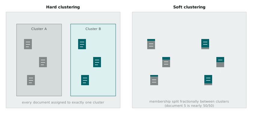
That right panel is the entire justification for using EM over a simpler approach like running k-means on term frequency vectors. k-means would force every document into one bucket, the same hard partition it forces on numeric data, and it would do so with no visibility into which documents it was unsure about. EM’s responsibilities matrix keeps that uncertainty on the record. A document with a responsibility close to 0.5 for two different clusters is not a modelling failure, it is a correct and informative answer, and it is one that a hard clustering method has no way to express at all.
What carries over from the earlier version
The mechanics are identical to the Gaussian case in every way that matters: guess parameters, compute responsibilities under those parameters, update the parameters weighted by those responsibilities, repeat until the log-likelihood stops moving. Only the shape of the thing being estimated changes, a mean and covariance for continuous data, a distribution over a vocabulary for text. That portability is what makes EM worth understanding properly rather than as a k-means variant. Once the E-step and M-step structure is genuinely understood rather than memorised for one data type, swapping in a different generative assumption for a different kind of data stops being a research problem and starts being an afternoon’s work.