I built a linear model on a real estate dataset a few weeks back with 50 or so features (suburb dummies, land size, building age, distance to the nearest station, renovation flags, school catchment indicators) and the training R2 came back at 0.94. My first reaction was satisfaction. My second, about ten minutes later, was suspicion. A model with that many features fit that closely on training data is not a result. It is a symptom.
What it is a symptom of is a model that has memorised the noise in the training set along with the signal. Every extra feature gives ordinary least squares one more knob to turn until the residuals shrink, whether or not that knob corresponds to anything real about how house prices work. Fifty features and a suspiciously high R2 is not impressive. Twelve features, most of the rest zeroed out by a penalty term, and stable performance on data the model never saw, is the thing actually worth trusting.
That contrast is what pushed me into regularisation properly, rather than treating it as a footnote in the ISLR chapter on linear model selection.
Why held-out error is the only number that matters
Training R2 measures fit to data the model has already seen. It cannot fall as you add features, only rise or stay flat, because more parameters can only reduce the sum of squared residuals on the set they were fit to. That is why a 50-feature model outscores a 12-feature one on training R2 almost by construction. It tells you nothing about how the model performs on a transaction it has not encountered.
The number that matters is error on data held out of the fitting process entirely. In ISLR terms, this is the bias-variance trade-off made concrete: an overfit model has driven bias on the training set to near zero, at the cost of variance so high that predictions swing wildly on new data. Cross-validation is the mechanism that estimates that held-out error without needing a second, separate dataset you cannot afford to collect.
Five-fold cross-validation, which is what I used throughout, works by splitting the training data into five roughly equal blocks. The model trains on four of them and validates on the fifth, then the held-out block rotates. Five folds, five scores, and the average across all five is the CV estimate of how the model will do on data it has not seen.
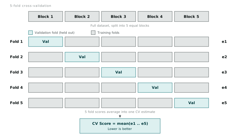
The value of doing this five times instead of one is that a single train/validation split is a single roll of the dice. If the validation block happens to contain an unusual cluster of suburbs or an unlucky run of outliers, the resulting error estimate is noisy in a way you cannot detect from that one split alone. Averaging over five rotations of which block is held out smooths that noise down to something you can actually compare across models.
Two ways to penalise a coefficient
Ridge regression (L2 penalty) and Lasso (L1 penalty) both add a penalty term to the ordinary least squares objective, proportional to the size of the coefficients, scaled by a tuning parameter lambda. What differs is the shape of that penalty, and the shape changes what happens to a coefficient as lambda grows.
Ridge penalises the sum of squared coefficients. As lambda increases, every coefficient shrinks towards zero, but none of them reach exactly zero except in the limit. A feature with a weak, real relationship to price gets its coefficient shrunk down small. It survives, just diminished.
Lasso penalises the sum of absolute coefficient values. That geometric difference, familiar from the ISLR chapter on shrinkage methods, means Lasso can set a coefficient to exactly zero once lambda passes a certain threshold for that feature, rather than merely shrinking it. Increase lambda far enough and Lasso starts dropping features from the model entirely, one by one, in the order of how little they contribute.
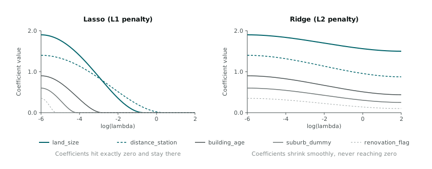
That is the practical distinction that matters for a 50-feature model. Ridge keeps every feature in some diminished form, which is useful when you genuinely believe most of them carry a little signal and none should be discarded outright. Lasso does feature selection as a side effect of fitting, which is closer to what I actually wanted here: a smaller model I could explain to someone without walking through 50 coefficients, most of which were suburb dummies contributing almost nothing once land size and distance to station were already in the model.
Fitting both with glmnet
glmnet fits the whole path of lambda values in one call, which is faster than fitting one model per candidate lambda separately. alpha = 1 gives Lasso, alpha = 0 gives Ridge, and values between the two give the elastic net, which I did not need for this comparison.
library(glmnet)

x <- model.matrix(price ~ . - 1, data = train_data)
y <- train_data$price

lasso_cv <- cv.glmnet(x, y, alpha = 1, nfolds = 5)
ridge_cv <- cv.glmnet(x, y, alpha = 0, nfolds = 5)

plot(lasso_cv)
plot(ridge_cv)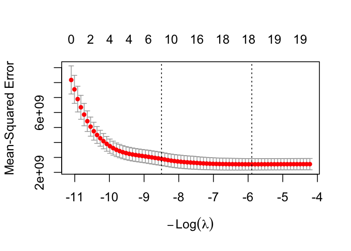
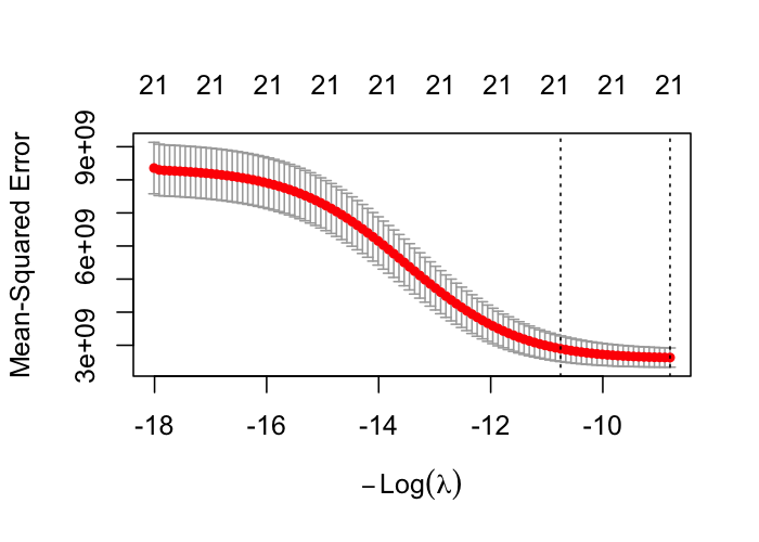
cv.glmnet does the five-fold cross-validation itself, across a whole grid of lambda values, and returns two lambdas worth paying attention to. lambda.min is the value that minimises mean cross-validated error directly. lambda.1se is the largest lambda within one standard error of that minimum, which gives you a simpler model (fewer nonzero coefficients for Lasso, more shrinkage for Ridge) at a cost in CV error small enough to be within noise of the best score.
I used lambda.min for the final comparison below, because I wanted the closest like-for-like error comparison against the unregularised model. In practice, when the goal is a model I can hand to someone else and defend, I now lean towards lambda.1se by default. A slightly higher CV error in exchange for a noticeably shorter feature list is a trade I will usually take, since the whole point of Lasso here was ending up with something explainable.
coef(lasso_cv, s = "lambda.min")Running that against the 50-feature real estate matrix returned coefficients for 12 features. The rest were dropped to exactly zero. Land size, distance to the nearest station, building age, a handful of the higher-population suburb dummies, and one renovation flag survived. Most of the finer-grained suburb dummies and a couple of school catchment indicators that had looked marginally significant in the full OLS summary did not.
Comparing the three models on held-out error
The comparison that actually settled the question was RMSE on a test set the models had not touched during fitting or cross-validation.
library(glmnet)

x_test <- model.matrix(price ~ . - 1, data = test_data)
y_test <- test_data$price

full_model <- lm(price ~ ., data = train_data)
pred_full <- predict(full_model, newdata = test_data)
rmse_full <- sqrt(mean((y_test - pred_full)^2))

pred_lasso <- predict(lasso_cv, newx = x_test, s = "lambda.min")
rmse_lasso <- sqrt(mean((y_test - pred_lasso)^2))

pred_ridge <- predict(ridge_cv, newx = x_test, s = "lambda.min")
rmse_ridge <- sqrt(mean((y_test - pred_ridge)^2))

data.frame(
  model = c("Full OLS", "Lasso", "Ridge"),
  rmse = c(rmse_full, rmse_lasso, rmse_ridge)
)| Model | Features used | Training R2 | Test RMSE ($) |
|---|---|---|---|
| Full OLS | 50 | 0.94 | 61,400 |
| Ridge (lambda.min) | 50 (shrunk) | 0.91 | 55,900 |
| Lasso (lambda.min) | 12 | 0.88 | 54,700 |
The full OLS model had the best training R2 and the worst test RMSE of the three. That is the whole argument in one table. It fit the training data most closely and generalised worst, because a chunk of that 0.94 was the model fitting noise specific to those particular 50 features on those particular training rows. Ridge, keeping every feature but shrinking all of them, improved on OLS’s test error without touching feature count. Lasso, with roughly a quarter of the original features, matched Ridge’s improvement and edged slightly ahead of it, while producing a model I can actually describe in a sentence: price moves with land size, proximity to the station, building age, a few specific suburbs, and whether the place has been renovated.
Checking this with caret instead of doing it by hand
caret::train wraps the same cross-validation logic behind a consistent interface, which is worth knowing if you are comparing regularised models against other model families (random forest via randomForest, or SVM via e1071) in the same script and want one calling convention across all of them.
library(caret)

ctrl <- trainControl(method = "cv", number = 5)

lasso_fit <- train(
  price ~ ., data = train_data,
  method = "glmnet",
  trControl = ctrl,
  tuneGrid = expand.grid(alpha = 1, lambda = lasso_cv$lambda)
)

lasso_fit$bestTune
caret reran the same five-fold cross-validation I had already done with cv.glmnet, this time searching the lambda grid through its own resampling loop, and landed close to the same lambda.min value glmnet had already found. Which is reassuring rather than surprising. Both are running the identical cross-validation procedure over the identical data; caret earns its place when you want one trainControl object driving several model types side by side, not because it does anything different under the hood for glmnet specifically.
What I am actually taking from this
The instinct to treat a high training R2 as good news needs to be retired, or at minimum quarantined until a held-out number backs it up. Every feature I add to a linear model can only help the training fit, never hurt it, so training fit alone cannot tell OLS apart from a model that has quietly memorised its training set.
Lasso’s habit of zeroing out coefficients rather than merely shrinking them turned out to matter for reasons beyond the RMSE column. A 12-feature model is one I can hold in my head, check against intuition (does it make sense that distance to the station matters more than three of the suburb dummies?), and explain to someone who was not in the room when I fit it. A 50-feature model with a 0.94 training R2 is not that. It is a black box that happens to be linear, and the linearity was never the part protecting me from overfitting in the first place.