I fit my first lm() on two variables, one predictor and one response, and had a coefficient, a p-value and a clean line through a scatterplot inside about four minutes. Fitting one on a real estate dataset with close to eighty features per property took considerably longer, mostly because the four-minute version never taught me what happens once half the columns are measuring the same underlying thing in slightly different units.
The dataset is residential property sales, one row per house, just under eighty columns: lot size, overall quality rating, basement finish type, garage capacity, number of bathrooms, roof material, neighbourhood, year built, year of last renovation, and on. It reads as straightforward in a data dictionary. It stops reading as straightforward the moment you try to say what any single coefficient actually means once the other seventy nine are sitting in the model with it.
Eighty features, three underlying stories
Square footage alone shows up four different ways in this data: above ground living area, total square footage including the basement, first floor square footage, and a derived total that sums several of the others. Garage size shows up as both an area in square feet and a car capacity. Number of rooms above ground correlates with above ground living area for the obvious reason that rooms take space. None of this breaks lm(). R will fit a model across all eighty columns without complaint and hand back a coefficient for every one of them.
What breaks is the assumption underneath the model: that each coefficient describes the effect of one feature while holding the others fixed. When two columns are different measurements of roughly the same thing, “holding the other fixed” is not an operation you can actually perform on this data. It is a sentence the model lets you say without it meaning much.
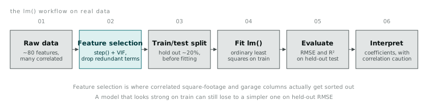
The stage that carries the most weight for a dataset shaped like this is feature selection, well before any evaluation metric enters the picture. Get that stage wrong and every number downstream, RMSE, R², the coefficient table, inherits the mistake.
Stepwise selection and the VIF check step() does not do
I start with the full model, every column that survived cleaning, fit against sale price.
houses <- read.csv("property_sales.csv", stringsAsFactors = TRUE)

# columns already cleaned of NAs and coerced to sensible types
full_fit <- lm(sale_price ~ ., data = houses)
That model fits. It also has 79 predictors on a dataset with a few thousand rows, which is more parameters than I want feeding into anything I plan to trust. MASS::stepAIC does the mechanical part of trimming that down, searching in both directions and keeping whatever combination of terms gives the lowest AIC at each step.
library(MASS)

step_fit <- stepAIC(full_fit, direction = "both", trace = FALSE)
length(coef(step_fit))
stepAIC brought the model from 79 predictors down to 24. What it will not tell you, because it is not built to, is whether any of the 24 that survived are still standing in for the same underlying property. AIC rewards a model for fitting well with fewer terms. It has no concept of “these two terms are measuring the same thing,” and a pair of correlated features can both look worth keeping by that criterion even though neither one, on its own, means what its coefficient suggests.
That is what car::vif() is for.
library(car)

vif_scores <- vif(step_fit)
sort(vif_scores, decreasing = TRUE)[1:6]| Feature | VIF |
|---|---|
| Above ground living area | 8.4 |
| First floor square footage | 7.9 |
| Total basement square footage | 6.1 |
| Garage area (sq ft) | 5.3 |
| Total rooms above ground | 4.7 |
| Overall quality rating | 3.2 |
The rule of thumb I use is that a VIF past 5 is worth a closer look and past 10 is a problem you cannot reasonably ignore. Above ground living area and first floor square footage sit at 8.4 and 7.9 for the same reason: on a single storey house, first floor square footage and above ground living area are close to the same number wearing two different column names. Keeping both does not add information. It splits one real signal across two coefficients and makes each one individually less trustworthy. I dropped first floor square footage and total rooms above ground, kept above ground living area as the single square footage measure and garage capacity in car count instead of area, and refit.
Train once, test on rows the model never saw
Everything so far ran on the full dataset, which is fine for exploring but tells you nothing about how the model behaves on a house it has not seen. Before fitting anything I plan to evaluate, I split.
set.seed(42)
n <- nrow(houses)
train_idx <- sample(seq_len(n), size = floor(0.8 * n))

train <- houses[train_idx, ]
test <- houses[-train_idx, ]
The reduced formula, nine predictors, refit on the training rows only.
final_fit <- lm(sale_price ~ gr_liv_area + overall_qual + total_bsmt_sf +
                   garage_cars + full_bath + year_built + lot_area +
                   dist_arterial_road + years_since_remodel,
                 data = train)
preds <- predict(final_fit, newdata = test)
rmse <- sqrt(mean((test$sale_price - preds)^2))
r2 <- cor(test$sale_price, preds)^2| Model | Predictors | Train RMSE | Test RMSE | Test R² |
|---|---|---|---|---|
| Full lm() | 79 | $17,900 | $33,640 | 0.79 |
| Stepwise (AIC) | 24 | $20,310 | $25,920 | 0.85 |
| Reduced (VIF-checked) | 9 | $22,480 | $24,150 | 0.87 |
The full model has the lowest training RMSE of the three and the worst test RMSE by a wide margin. That is the overfitting story you would expect from 79 parameters on this many rows, but the multicollinearity makes it worse than a plain parameter count would suggest. Correlated columns give the optimiser several near-equivalent ways to carve up the same variance, and it picks whichever split fits the training noise best. None of those splits are the “true” relationship, so none of them hold up on the test set.
The reduced model has the highest training RMSE of the three, which on a training-only view looks like the weakest fit. It has the lowest test RMSE and the highest test R². Nine honest predictors, chosen to avoid measuring the same thing twice, generalise better than 79 that include several redundant ones. I would rather report the model that looks slightly worse on the numbers I fit it with and better on the numbers that matter.
What a coefficient means when everything is correlated
In the full model, the coefficient on total basement square footage came out negative. Read plainly, that says more basement space lowers sale price, which is not a claim I believe about this market or any other. What is actually happening is that above ground living area, the larger and more correlated square footage measure, is already in the model soaking up most of that shared variance. The basement term is left to explain whatever is left over once the bigger feature has taken its share, and what is left over is not guaranteed to have the sign you would expect from the raw feature on its own.
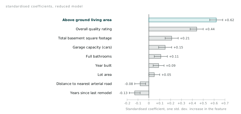
| Feature | Standardised coefficient | 95% CI |
|---|---|---|
| Above ground living area | +0.62 | [0.56, 0.68] |
| Overall quality rating | +0.44 | [0.38, 0.50] |
| Total basement square footage | +0.21 | [0.15, 0.27] |
| Garage capacity (cars) | +0.15 | [0.09, 0.21] |
| Full bathrooms | +0.11 | [0.05, 0.17] |
| Year built | +0.09 | [0.04, 0.14] |
| Lot area | +0.05 | [0.00, 0.10] |
| Distance to nearest arterial road | -0.08 | [-0.13, -0.03] |
| Years since last remodel | -0.13 | [-0.18, -0.08] |
Standardising the coefficients (each feature centred and scaled before fitting) is the only way I have found to put them on a chart together without garage capacity, measured in whole cars, looking meaningless next to lot area, measured in thousands of square feet. It does not fix the correlation problem. It just makes the relative sizes readable. “Holding everything else constant” is the phrase every regression textbook uses to explain a coefficient, and on a dataset where above ground living area, total basement square footage and total rooms above ground move together in almost every real house, there is no version of the data where you hold two of them fixed and vary the third. The phrase describes a thought experiment the data cannot run.
The line through square footage does not stay straight
The other assumption the textbook examples lean on is that the relationship between the strongest predictor and the outcome is roughly linear across its whole range. Plotting sale price against above ground living area on its own, before any of the other columns get involved, backs that up only up to a point. The relationship looks close to linear out to around 3,000 square feet. Past that, the slope flattens. An extra 500 square feet on a 1,800 square foot house moves the price by more than the same 500 square feet added to a 4,000 square foot house, and a single global slope coefficient cannot represent both of those at once. It reports something like the average of the two, which describes neither well.
Renovation timing does something similar in a different shape. Sale price against years since the property was last remodelled is not a smooth decline. Houses remodelled within the last year or two cluster at a premium, and the drop-off after that is closer to a step than a slope, because a remodel resets a buyer’s perception of the property’s condition in a way that does not fade gradually year by year, it holds until the next visible sign of age shows up. A linear term on years since remodel captures the general downward direction and misses the shape entirely.