I had two candidate regression models for the same dataset a few weeks ago, one with four predictors and one with seven, and both came back from summary() with every coefficient significant at the 0.05 level. That result told me nothing about which model I should actually use. Significance testing answers a question about individual coefficients, one at a time, against a null hypothesis of zero effect. It has no built-in opinion about whether the seven-variable model is worth its extra complexity over the four-variable one. I went looking for a criterion that could actually compare the two models against each other, not each coefficient against zero, and that search is what pulled me toward AIC, BIC, and eventually Minimum Message Length.
The question a p-value actually answers
The American Statistical Association put out a formal statement on p-values back in March, and reading it was the first time I had seen, in writing, from a body with that much institutional weight behind it, an admission of exactly the discomfort I already had with the metric. A p-value is the probability of seeing data this extreme, or more extreme, if the null hypothesis were true. That is a narrow, specific claim. It is not the probability that the null hypothesis is true. It is not a measure of effect size. It is not, on its own, a statement about how well a model explains the data relative to a competing model.
Stepwise selection built on p-values compounds the problem. Add or remove variables one at a time based on whether each crosses the 0.05 threshold, and you are running dozens of significance tests against the same dataset without correcting for the fact that you are running dozens of tests. The final model that survives that process tends to look better on this dataset than it will on the next one, because some of what got kept was noise that happened to clear the bar by chance. I had been doing a version of this by hand, adding a predictor, checking if its p-value looked respectable, keeping it if so, for longer than I want to admit.
AIC and BIC: penalising complexity directly
Akaike’s Information Criterion and the Bayesian Information Criterion both start from a different premise. Instead of asking whether one coefficient differs from zero, they ask how well the whole model explains the data, adjusted by a penalty for how many parameters it took to get there.
fit_small <- lm(mpg ~ wt + hp, data = mtcars)
fit_large <- lm(mpg ~ wt + hp + disp + qsec + drat + cyl, data = mtcars)

AIC(fit_small, fit_large)
BIC(fit_small, fit_large)
AIC is 2k - 2*log-likelihood, where k is the number of parameters. BIC replaces the 2k term with k*log(n), which means the penalty for adding a parameter grows with sample size rather than staying fixed. In practice this makes BIC pickier than AIC as your dataset gets larger, and it is why the two criteria sometimes disagree about which model to prefer. Lower is better for both. Running AIC() and BIC() side by side on the two mtcars fits above, the larger model rarely wins on either once the penalty is applied, even though every one of its extra coefficients looked significant on its own.
step() in base R can drive a model search using AIC as the selection criterion instead of p-values, step(fit_large, direction = "backward"), and the difference in behaviour compared to hand-rolled p-value stepping is noticeable. AIC-based selection is still not free of the multiple-comparisons issue that plagues stepwise regression generally, but at least it is optimising for something closer to what I actually care about: a model that explains the data well without paying for parameters it does not need.
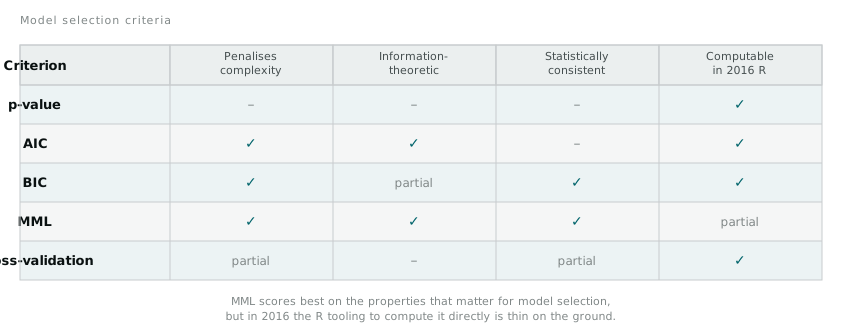
BIC has a property AIC lacks, called consistency: as the sample size grows toward infinity, BIC will select the true model with probability approaching one, assuming the true model is among the candidates. AIC does not have that guarantee, and is known to favour slightly larger models than necessary even asymptotically. That single difference is enough reason to reach for BIC over AIC whenever I actually believe one of my candidate models is close to correct, and to reach for AIC when I am more interested in prediction than in recovering the true generating process.
Minimum Message Length: the same idea taken further
Reading around AIC and BIC eventually led me to Minimum Message Length, developed originally by Chris Wallace, an Australian computer scientist working through the late 1960s and into the following decades. MML frames model selection as a communication problem. Imagine you need to send someone your dataset over a wire, and you are paying by the bit. You can send the raw numbers directly, or you can send a description of a model plus the small corrections needed to reconstruct the exact data from that model’s predictions. The best model, under MML, is whichever choice makes that total message, model description plus residual corrections, the shortest.
A simple model is cheap to describe but leaves large corrections, because it does not explain much of the data’s structure. An extremely complex model can shrink the corrections almost to nothing, but the model description itself becomes expensive, because you need more bits to specify more parameters, each to some precision. The message length is a sum of both costs, and the model that minimises it is one that has genuinely earned its complexity rather than one that has merely memorised the training data.
What I like about that framing over AIC and BIC is that it does not depend on the sample size growing to infinity to make sense, and it is not tied to a specific fixed penalty formula in the way AIC’s 2k is. It handles model comparisons that AIC and BIC struggle with, comparing models with entirely different structures rather than just different numbers of parameters within the same family. It also matches, more directly than either information criterion, the intuition I actually had about the four-variable versus seven-variable regression: the extra three variables in the larger model needed to earn their keep by shrinking the unexplained error by more than it cost to describe them, and on my data they did not.
The honest caveat is that direct MML tooling in R, as of this year, is thin. There is no equivalent of calling AIC() on a fitted lm() object and getting a message length back. Working with the idea in practice, for now, means either implementing the two-part code calculation by hand for a specific model family or treating MML as a way of thinking about the AIC and BIC numbers I already have, rather than as a fourth number I can compute directly.
Where regularisation fits in
L1 and L2 regularisation sit on the same spectrum as all of this, even though they are usually framed as separate from model selection. Ridge regression, L2, shrinks every coefficient toward zero without setting any of them exactly to zero, trading a small amount of bias for a reduction in variance. Lasso, L1, can shrink coefficients all the way to zero, which means it performs variable selection as a side effect of fitting the model rather than as a separate stepwise procedure.
library(glmnet)

x <- as.matrix(mtcars[, c("wt", "hp", "disp", "qsec", "drat", "cyl")])
y <- mtcars$mpg

cv_fit <- cv.glmnet(x, y, alpha = 1)  # alpha = 1 is lasso, 0 is ridge
coef(cv_fit, s = "lambda.min")
cv.glmnet() picks the penalty strength, lambda, by cross-validation rather than by a fixed formula, which puts it in the same family as the other approaches here: none of these methods take complexity for granted, they all make it pay for itself somehow, whether through an explicit penalty term, an information-theoretic message length, or held-out prediction error.
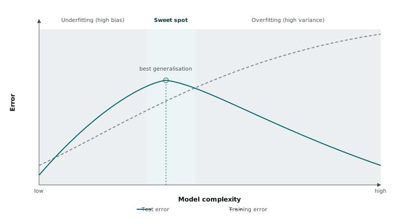
That U-shaped curve is the shape every one of these criteria is trying to locate from a different angle. Training error keeps falling as complexity increases, because a sufficiently flexible model can always fit the training data more closely, whether or not the extra flexibility reflects anything real. Test error falls, then rises again, because past some point the extra flexibility is fitting noise specific to the training sample rather than structure that will generalise. p-values, taken one coefficient at a time, have no view of this curve at all. AIC, BIC, MML, and cross-validation are all, in their own way, trying to find the bottom of it.
I still report p-values when someone asks whether an individual effect is distinguishable from noise, because that is a question they genuinely answer. I no longer use them to decide between two whole models. For that comparison, AIC and BIC give me a number I can act on today, and MML gives me a clearer picture of what that number is actually trying to measure: not surprise under a null hypothesis, but the shortest honest description of the data I can find.