I tried to optimise a delivery route order for a small set of stops a few weeks ago, and reached for the same instinct I use for most fitting problems: take a derivative, find where it is zero, done. There is no derivative here. A route order is a permutation, one of a discrete, finite, but enormous set of possible orderings, and there is no smooth surface connecting one ordering to the next that calculus can walk down. Swap two stops and the total distance jumps by some amount that has nothing to do with a gradient, because there is no continuous path between “visit A then B” and “visit B then A.” Calculus assumes you can nudge a solution by an infinitesimal amount and see how the outcome responds. A permutation cannot be nudged.
That gap is where Monte Carlo methods and simulated annealing earn their place. Neither needs a gradient. Both trade a mathematical guarantee for a practical one: given enough random sampling, structured the right way, you will land somewhere close to a good answer, even when you cannot write down the shape of the space you are searching.
Monte Carlo, in the plain sense
The core idea behind Monte Carlo methods is older and simpler than most of what gets built on top of it: if you cannot solve a problem analytically, simulate it many times and let the law of large numbers do the work. Estimating an integral you cannot solve in closed form, sample randomly under the curve and count the proportion that falls below it. Estimating an expected value for a process too complicated to write down as an equation, run the process thousands of times with random inputs and average the outcomes.
n <- 100000
x <- runif(n, -1, 1)
y <- runif(n, -1, 1)
inside_circle <- (x^2 + y^2) <= 1
pi_estimate <- 4 * mean(inside_circle)
pi_estimate
This particular example, estimating pi from the proportion of random points landing inside a unit circle, is the textbook illustration, and running it in R takes about four lines. What it demonstrates matters more than the party trick: a problem with no algebraic shortcut can still be answered numerically, to a precision that improves as you throw more random samples at it. That principle, simulate rather than solve, is the seed that both simulated annealing and genetic algorithms grow out of.
Where the loss surface stops being smooth
Gradient-based optimisation, the kind behind optim()’s default methods like BFGS or the workhorse of every regression fit, assumes the function you are minimising is differentiable, or at least well-approximated by something differentiable nearby. That assumption holds for a huge share of statistical modelling. It falls apart in two common situations.
The first is a discrete search space, where solutions are permutations, subsets, or combinations rather than points on a continuous number line. The travelling salesman problem, finding the shortest route visiting a set of cities exactly once, is the classic example, and it is NP-hard in general, meaning no known algorithm solves it exactly in reasonable time as the number of cities grows.
The second is a continuous space that is non-convex and riddled with local optima, where a gradient method starting from the wrong point will confidently walk downhill into a valley that is nowhere near the best one available. Gradient descent has no mechanism for climbing back out once it has settled, because by definition it only ever moves in the direction that currently looks best.
Simulated annealing: accepting worse moves on purpose
Simulated annealing solves the local-optimum problem with an idea borrowed directly from metallurgy. Heating a metal and cooling it slowly lets its atoms settle into a low-energy, structurally sound arrangement, because at high temperature the atoms have enough energy to jump out of a poor local configuration, and as the temperature drops that freedom shrinks, locking the structure into whatever arrangement it has found by the time it cools.
The algorithm mirrors that physical process directly. Start with a candidate solution and a high “temperature.” At each step, propose a small random change to the current solution, and decide whether to accept it using the Metropolis criterion: if the change makes things better, always accept it; if it makes things worse, accept it anyway with probability exp(-Δ / T), where Δ is how much worse the new solution is and T is the current temperature. Then reduce the temperature according to some cooling schedule and repeat.
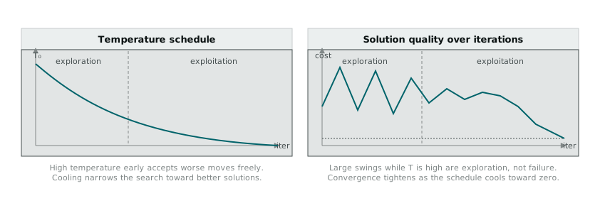
Early on, with temperature high, the algorithm accepts a lot of moves that make the solution temporarily worse, which is exactly what lets it escape a local optimum that a purely greedy search would get stuck in. That phase looks noisy if you plot solution quality against iteration, jumping up and down as it explores. As the temperature drops, the probability of accepting a worse move shrinks toward zero, and the algorithm settles into refining whatever region of the search space it has found itself in by that point. Too fast a cooling schedule and it locks in early, before it has explored enough. Too slow and it wastes a lot of iterations on moves that barely matter anymore.
R has this built in as one of the methods for optim(), which surprised me the first time I noticed it in the documentation.
result <- optim(par = initial_guess, fn = cost_function,
                 method = "SANN",
                 control = list(maxit = 10000, temp = 10))
method = "SANN" runs simulated annealing instead of a gradient method, useful for exactly the non-convex continuous problems described above, though it is a fairly basic implementation without much control over the cooling schedule beyond a starting temperature and iteration count. For discrete combinatorial problems like a route ordering, I ended up writing the accept-or-reject loop by hand, since optim()’s built-in SANN expects a numeric parameter vector rather than a permutation.
tour <- sample(n_cities)
temp <- 100
cooling <- 0.995

for (i in 1:5000) {
  swap <- sample(n_cities, 2)
  candidate <- tour
  candidate[swap] <- candidate[rev(swap)]

  delta <- tour_length(candidate, dist_matrix) - tour_length(tour, dist_matrix)
  if (delta < 0 || runif(1) < exp(-delta / temp)) {
    tour <- candidate
  }
  temp <- temp * cooling
}
Running this against a random starting tour and against a greedy nearest-neighbour heuristic on the same set of cities made the difference concrete rather than theoretical.
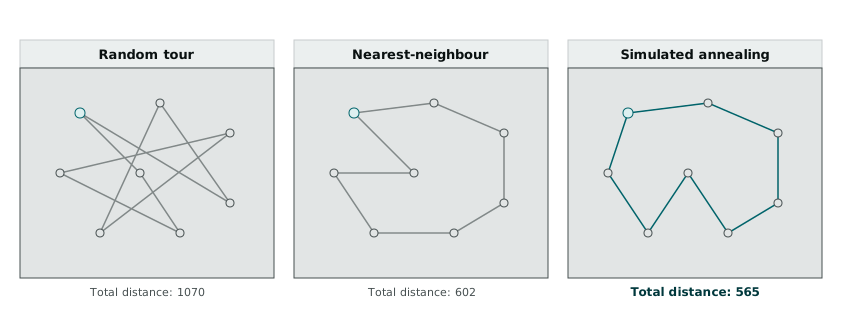
The random tour is what you get with zero intelligence applied, stops visited in whatever order they happened to be drawn, and the total distance reflects that, crossing back and forth across the map with no regard for proximity. The nearest-neighbour heuristic, always jump to whichever unvisited city is closest, does far better with almost no computation, but it has a known weakness: greedy local choices early on can strand it with an expensive final leg back to wherever it started, because nothing in the heuristic looks ahead. Simulated annealing, given enough iterations, found a tour shorter than either, because its willingness to accept temporarily worse swaps let it escape the kind of arrangement the greedy heuristic gets locked into.
Genetic algorithms and the population alternative
Genetic algorithms attack the same class of problem from a different direction, maintaining a whole population of candidate solutions rather than a single one, and evolving that population through selection, crossover, and mutation across generations. The genalg package, which needs R 3.2.1 or later, is the one I have been using for this in R.
library(genalg)

evaluate <- function(x) {
  selected <- which(x == 1)
  if (length(selected) == 0) return(Inf)
  model <- lm(y ~ ., data = df[, c(selected, ncol(df))])
  -summary(model)$adj.r.squared
}

result <- rbga.bin(size = ncol(df) - 1, evalFunc = evaluate,
                    popSize = 100, iters = 200,
                    mutationChance = 0.05)
rbga.bin() works on binary-encoded chromosomes, where each gene is a 1 or 0 deciding whether to include a given variable. That maps to feature selection almost exactly: the chromosome is a mask over the columns, and the fitness function fits a model on whichever subset the mask selects. For permutation-style problems like the travelling salesman, a binary string does not obviously encode a valid tour, and simulated annealing is more straightforward to reason about, since the accept-or-reject rule for a single candidate swap is simpler to implement correctly than crossover operators that need to produce valid permutations from two parent permutations.
A related idea worth not confusing with the others
Markov Chain Monte Carlo shares the Metropolis acceptance rule with simulated annealing, and it is easy to blur the two together the first time you meet both. The distinction that matters: simulated annealing is trying to find the single best solution, and it uses a cooling temperature specifically so it eventually stops exploring and commits to one answer. MCMC is trying to sample from an entire probability distribution, usually a posterior distribution in a Bayesian model, and it deliberately keeps exploring forever, because the goal is a representative sample of the whole distribution’s shape, not a single point estimate. Same acceptance mechanics, opposite goals. Confusing them for a while, before the distinction clicked, cost me an afternoon staring at a Metropolis-Hastings sampler wondering why it kept “wandering” instead of settling down. It was never supposed to settle down.
None of these methods come with a guarantee. Simulated annealing can still miss the global optimum if the cooling schedule is wrong. A genetic algorithm’s population can converge prematurely to a mediocre solution if selection pressure is too aggressive too early. What they offer instead of a guarantee is a way to make progress on problems where gradient descent has nothing to grab onto, discrete search spaces and non-convex surfaces that show up constantly in scheduling, routing, and combinatorial selection problems, long after the neat, differentiable version of the same problem has already been solved by something faster.