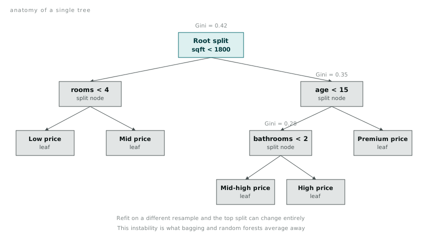
I fit the same rpart tree twice last week on a housing price dataset, once on the full training set and once after dropping a random 20% of rows. The top split changed. First run, the tree split on square footage before anything else. Second run, number of bedrooms went first, and square footage did not show up until the second level. Nothing else about the data or the code changed. Only which rows happened to be in the sample.
That is the property of a single tree that took me longer than it should have to take seriously. A tree is easy to read: follow the splits down to a leaf and you have an explanation you could put in front of someone who has never heard of machine learning. It is also unstable in a way that linear models are not. A regression coefficient moves a little when you resample. A tree’s structure can move a lot, because an early split near a tie between two candidate variables can flip either way depending on which rows happen to be present, and everything below that split inherits the change.
Why a single tree overfits
rpart builds a tree by recursive partitioning: at each node, it searches every variable and every possible split point for the one that most reduces impurity in the resulting two child nodes, then repeats inside each child. Left alone, it keeps splitting until nodes are pure or too small to split further, which means it will happily carve out a leaf for a single outlier house if nothing stops it.
library(rpart)
library(rpart.plot)

tree_fit <- rpart(price ~ sqft + bedrooms + bathrooms + age + lot_size + suburb,
                   data = train,
                   method = "anova",
                   control = rpart.control(cp = 0.01, minsplit = 20))

rpart.plot(tree_fit, type = 2, extra = 101, box.palette = "Greens")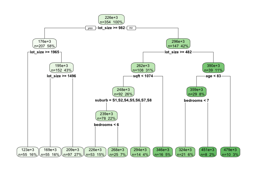
The cp (complexity parameter) argument keeps this in check. It sets the minimum improvement a split must deliver before rpart bothers making it. I ran printcp(tree_fit) and picked the cp value with the lowest cross-validated error rather than the lowest training error, because training error only ever goes down as the tree grows.
Even with cp tuned properly, the instability problem does not go away. A tuned tree still picks one path through the variables at each split, and that path is sensitive to which rows are in front of it.
Bagging: average away the instability
Bootstrap aggregating, bagging, is the direct answer to instability. Draw a bootstrap sample from the training data (same size, sampled with replacement, so some rows appear more than once and some are left out entirely), fit a full tree on it, and repeat several hundred times. To predict a new point, average the predictions across all the trees (for regression) or take a majority vote (for classification).
Each individual tree in a bagged ensemble is still unstable on its own. What changes is that the average of several hundred unstable trees is far more stable than any one of them, the same way the mean of several hundred noisy measurements beats any single measurement. The variance that made a single tree unreliable gets averaged down.
I did not spend much time on bagging in isolation, because random forests are a near-free improvement on it. Random forests are bagging plus one more idea.
Random forests: decorrelating the trees
Bagged trees are not independent of each other. If one variable is a genuinely strong predictor, most bootstrap trees will use it for the first split regardless of which rows they were trained on, because it dominates every sample. That correlation between trees caps how much variance reduction averaging can buy. Averaging correlated things helps less than averaging independent things.
Random forests break that correlation by restricting each split to a random subset of the available variables, chosen fresh at every split rather than once per tree. The size of that subset is mtry. A strong predictor no longer dominates every tree, because at a given split it might not even be one of the candidates on offer. Individual trees get a little worse. The forest as a whole gets more stable, because the trees disagree with each other in more useful ways.
library(randomForest)

rf_fit <- randomForest(price ~ sqft + bedrooms + bathrooms + age + lot_size + suburb,
                        data = train,
                        ntree = 500,
                        mtry = 3,
                        importance = TRUE)

print(rf_fit)
print(rf_fit) reports the out-of-bag (OOB) error alongside the fit, and this is one of the more useful things about a forest over a single tree. Because each tree trains on a bootstrap sample, roughly a third of the training rows are left out of any given tree, the “out-of-bag” rows for that tree. Every row therefore has predictions from the subset of trees that never saw it, which gives an honest estimate of test error without holding out a separate validation set.
rf_fit$mse[rf_fit$ntree]
sqrt(rf_fit$mse[rf_fit$ntree])
That last line gives OOB RMSE directly from the fitted object. I still keep a proper held-out test set for the final comparison across model types, but during mtry tuning the OOB error is nearly free, and I lean on it rather than running repeated cross-validation.
The trade the forest makes for that stability is the one I keep coming back to: you cannot look at a random forest and explain a single prediction the way you trace a path down one tree. Five hundred trees voting is not something you sketch on a whiteboard. What a forest gives back instead is variable importance, aggregated across every tree.
importance(rf_fit)
varImpPlot(rf_fit, main = "Variable importance, random forest")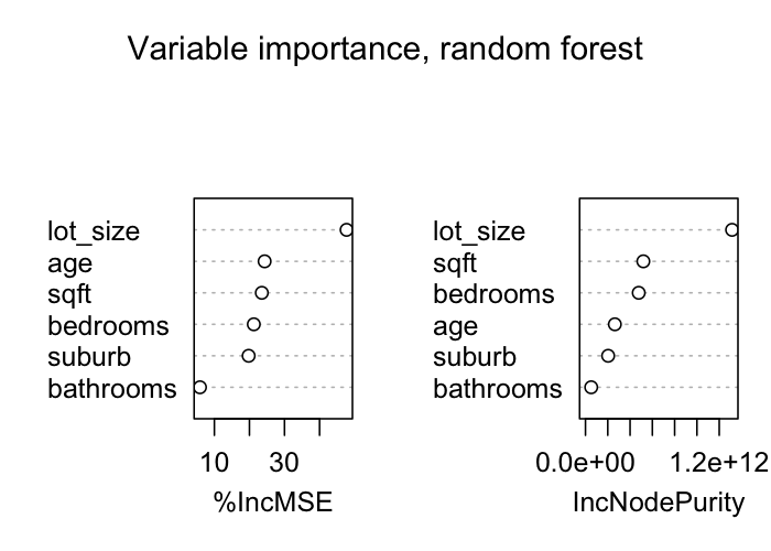
importance() reports two measures per variable: mean decrease in accuracy when its values are permuted across the OOB rows, and mean decrease in node impurity from splits on it across all trees. They usually agree on ranking but not always, and I trust %IncMSE (the permutation measure) more, because impurity reduction is biased towards variables with more possible split points, favouring continuous variables like sqft over categorical ones like suburb even when the categorical variable carries real signal.
| Variable | %IncMSE | IncNodePurity |
|---|---|---|
| sqft | 42.8 | 1,842,300 |
| suburb | 31.4 | 1,205,900 |
| bathrooms | 24.1 | 892,400 |
| age | 18.6 | 640,100 |
| bedrooms | 15.2 | 511,700 |
| lot_size | 12.9 | 448,300 |
This is the honest version of what a single tree’s top split gave me for free. The tree told me square footage mattered because it was the first split. The forest tells me square footage matters, and roughly how much relative to five other variables, averaged over enough resamples to trust the ranking. What it does not give back is the picture.
Boosting: fitting the mistakes, not the data
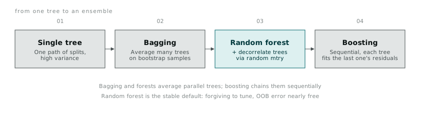
Random forests, and bagging underneath them, are parallel: every tree grows independently, on its own resample, and the ensemble only combines them at the end. Boosting via gbm is sequential, and that took me a while to get comfortable with conceptually.
A boosted model starts with a weak, deliberately shallow first tree, then looks at the residuals, the gap between its predictions and the actual values. The second tree fits not the original target but those residuals, trying to correct what the first tree got wrong. The third tree fits the residuals left after trees one and two, and so on. Each new tree is small, and each is chasing the error of everything before it rather than casting an independent vote.
library(gbm)

gbm_fit <- gbm(price ~ sqft + bedrooms + bathrooms + age + lot_size + suburb,
                data = train,
                distribution = "gaussian",
                n.trees = 3000,
                interaction.depth = 3,
                shrinkage = 0.01,
                cv.folds = 5,
                verbose = FALSE)

best_iter <- gbm.perf(gbm_fit, method = "cv")
The three parameters that matter most are n.trees, shrinkage, and interaction.depth. shrinkage scales down each tree’s contribution, so a low value like 0.01 forces the ensemble to learn slowly and needs more trees to get anywhere, but tends to generalise better than a fast-learning fit that overfits the residuals quickly. interaction.depth caps how many-way an interaction each tree can capture; I left it at 3 rather than the depth-1 stumps some references default to, because there were plausible two and three-way interactions between location and size variables I wanted the trees to reach. gbm.perf() with method = "cv" picks the number of trees minimising cross-validated error, because a boosted model with too many trees keeps reducing training error long after it has stopped helping on new data. A different failure mode to a single overgrown tree, but still overfitting.
Comparing all four on held-out data
Same train/test split, same predictors, four fitted models: the single rpart tree, the random forest, the gbm boosted model, and a radial-kernel SVM via e1071 as a non-tree comparison point.
svm_fit <- svm(price ~ sqft + bedrooms + bathrooms + age + lot_size + suburb,
               data = train,
               kernel = "radial",
               cost = 1)

rmse <- function(actual, predicted) sqrt(mean((actual - predicted)^2))

tree_pred <- predict(tree_fit, newdata = test)
rf_pred   <- predict(rf_fit, newdata = test)
gbm_pred  <- predict(gbm_fit, newdata = test, n.trees = best_iter)
svm_pred  <- predict(svm_fit, newdata = test)

rmse(test$price, tree_pred)
rmse(test$price, rf_pred)
rmse(test$price, gbm_pred)
rmse(test$price, svm_pred)| Model | Test RMSE | Rank |
|---|---|---|
Single tree (rpart) | 48,120 | 4 |
SVM, radial kernel (e1071) | 41,760 | 3 |
Random forest (randomForest) | 36,940 | 2 |
Boosted trees (gbm) | 34,280 | 1 |
The ordering is not a surprise on this kind of tabular data. The single tree, with one path of splits to overfit or underfit through, is the weakest of the four. The SVM does better by finding a smoother, more global decision surface, but lags both ensembles. Random forest and boosting land closest together, and which one wins tends to come down to the dataset and how much tuning time went into the gbm grid, more than any structural reason to expect boosting to win every time.
What the RMSE table does not show is how differently the two ensembles get there. The forest builds five hundred independent, high-variance trees and leans on averaging to cancel out their mistakes. Boosting builds a much smaller number of deliberately weak trees, each correcting the last one’s specific errors. Same broad idea, many trees beat one tree, opposite mechanism for getting there.
What I would reach for by default
If interpretability is the actual requirement, a single tree is still the right tool, not because it performs well, but because a client-facing explanation sometimes matters more than three RMSE points. For anything where the prediction itself is the product and nobody downstream needs to see the splits, I default to a random forest first because mtry and ntree are forgiving to tune and OOB error means I am not burning a validation set to check my work as I go. I reach for gbm when the forest has plateaued and I have time to tune shrinkage and interaction.depth properly, because a well-tuned boosted model has, on every dataset I have tried this on so far, come out ahead of the forest by a small but consistent margin. I have not found a dataset yet where the SVM beat both tree ensembles, though I suspect that says more about the kinds of tabular data I work with than about SVMs in general.