I had a k-nearest-neighbours model that would not stop recommending the same handful of customers, regardless of which customer I queried against. The bug took an embarrassingly long time to find: one feature was annual income, in dollars, ranging up to $300,000, and another was years as a customer, ranging from 0 to 12. Euclidean distance does not know that a $10,000 difference in income and a 10 year difference in tenure are meant to carry comparable weight. It just sees the numbers, and a difference in the thousands swamps a difference in single digits every time. The model was not broken. It was doing exactly what I told it to do, which was ignore tenure almost entirely.
That was the moment scaling stopped being a checkbox step I ran out of habit and became something I thought about deliberately, feature by feature.
Three ways to scale, and why they are not interchangeable
Min-max scaling squeezes every value into a fixed range, usually 0 to 1:
from sklearn.preprocessing import MinMaxScaler

scaler = MinMaxScaler()
df[['income_scaled']] = scaler.fit_transform(df[['income']])
It is easy to explain and it guarantees a bounded output, which some algorithms expect. Its weakness is exactly the outlier problem from the taxonomy piece I wrote a few weeks back: the scaling is anchored to the minimum and maximum observed values, so a single extreme point stretches the range and compresses everything else toward one end.
Z-score standardisation centres the data on a mean of 0 with a standard deviation of 1:
from sklearn.preprocessing import StandardScaler

scaler = StandardScaler()
df[['income_scaled']] = scaler.fit_transform(df[['income']])
This is less sensitive to a single outlier than min-max, because the mean and standard deviation, while still affected by outliers, do not clamp the output to a fixed range the way min and max do. It is the default I reach for with linear models and anything regularised, because the assumption of roughly comparable variance across features lines up with how those algorithms are actually penalising coefficients.
Robust scaling uses the median and interquartile range instead of the mean and standard deviation:
from sklearn.preprocessing import RobustScaler

scaler = RobustScaler()
df[['income_scaled']] = scaler.fit_transform(df[['income']])
Median and IQR barely move when you add one extreme value, which is the entire point. The five ordinary values in a column keep good spread relative to each other, and the outlier ends up with a large scaled value that clearly signals “unusual,” rather than being squashed against the edge of a 0 to 1 range or dragging the rest of the distribution toward it.
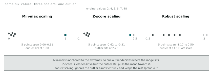
Running the same six values (2, 4, 5, 6, 7, 48) through all three methods makes the difference concrete. Min-max crushes the five ordinary points into the bottom 11 percent of the range, because the outlier alone defines where 1.0 sits. Z-score is a bit better, the ordinary points span a wider slice of the standardised range, but the outlier still pulls the mean toward it, which shifts everyone else’s score. Robust scaling barely notices the outlier is there: the five ordinary points keep a healthy spread relative to each other, and the outlier’s robust score lands far outside that range, which is arguably a more honest signal than either of the other two methods gives you.
None of the three is universally correct. If I am about to run PCA, where the objective actively depends on variance, z-score is close to mandatory. If the column is known to be outlier-heavy and I want the bulk of the distribution to keep useful structure, robust wins. If I need a bounded [0, 1] input because that is what an algorithm expects, min-max is the only one of the three that actually guarantees it.
Discretisation trades a number for a category, on purpose
Sometimes the right move is not to scale a continuous variable but to cut it into bins. Age becomes an age bracket. Income becomes an income tier. This throws away information, a 34 year old and a 38 year old become indistinguishable if the bins are five years wide, and I only do it when there is a reason to think the relationship between the variable and the outcome is not smooth, or when a bucketed version is what a downstream report actually needs to be readable.
Equal-width binning divides the range into bins of the same size:
df['age_bucket'] = pd.cut(df['age'], bins=5)Equal-frequency binning instead divides the data so each bin holds roughly the same number of rows, which matters when the distribution is skewed and equal-width bins would leave most of the data crammed into one bucket:
df['income_bucket'] = pd.qcut(df['income'], q=5)I default to qcut for anything income-like, because income distributions are skewed enough that equal-width bins put 80 percent of customers in the lowest bracket and leave the top bracket almost empty. cut earns its place when the bin boundaries need to mean something specific to a person reading the output, like age brackets that match a marketing segmentation someone already uses.
Sampling decides what the model even sees
Before any of the scaling or binning choices matter, there is a decision that happens earlier and gets less attention: how the data was sampled in the first place. A random train/test split is the default, and the right one most of the time:
from sklearn.cross_validation import train_test_split

X_train, X_test, y_train, y_test = train_test_split(
    X, y, test_size=0.3, random_state=42
)
It stops being the right default the moment the target class is imbalanced. A fraud dataset with 2 percent positive cases, split randomly, can hand the model a training set where the positive class barely appears in some folds, and a model that predicts “not fraud” every single time still scores 98 percent accuracy while being completely useless. Stratified sampling keeps the class ratio consistent between train and test:
from sklearn.cross_validation import StratifiedShuffleSplit

sss = StratifiedShuffleSplit(y, n_iter=1, test_size=0.3, random_state=42)
train_idx, test_idx = next(iter(sss))
That fixes the split, not the imbalance itself. Whether to also oversample the minority class, undersample the majority, or leave the imbalance in place and change the evaluation metric instead is a separate decision, and I have gone back and forth on it depending on the project. My rule of thumb now is to leave the training distribution alone and change what I measure, precision and recall instead of accuracy, or a cost-weighted loss function, before I reach for resampling. Resampling changes what the model has learned to expect, and that has bitten me once with a model that performed brilliantly on a resampled validation set and much worse once it saw the true, imbalanced production traffic.
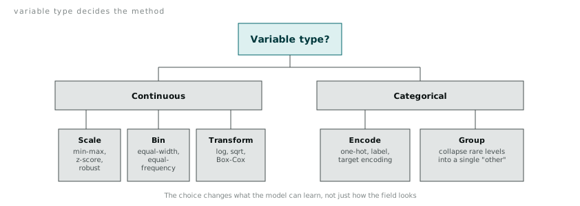
These are not preprocessing, they are modelling decisions
I used to think of scaling, binning, and sampling as things that happened before the real work, a chore to get through so the actual model could start. I do not think that any more. Every choice in this piece changes what the model is mathematically able to learn. Pick min-max over robust scaling on an outlier-heavy column and a linear model’s coefficients shift. Pick equal-width over equal-frequency binning on a skewed variable and you have effectively decided that most of your data does not matter. These decisions sit inside the model as much as the algorithm choice does. They are just made earlier, and get called something less important.