I spent three weeks this month on a project where the actual modelling took four days. The rest went into working out which of the 40,000 rows I could trust. A sensor feed had gaps that were not random, a join brought in duplicate customer records under three different spellings, and a handful of rows had values that were technically valid (an age of 150, a negative price) but obviously wrong. None of this was unusual. It is the normal shape of a real dataset, and not having a systematic way to work through it is the main reason cleansing projects run long.
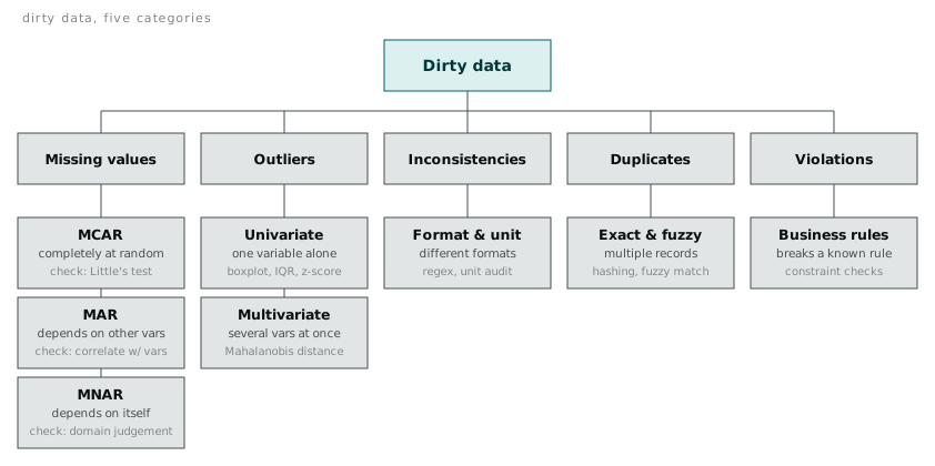
The taxonomy below is not exotic. Most of it comes from standard data quality thinking, but writing it down properly changed how I approach a new dataset. Instead of poking around until something looks wrong, I now check each category in order.
Missing values are not one problem
The mistake I made early on was treating every blank cell the same way: dropping the row, or filling it with the mean, and moving on. That works sometimes and quietly wrecks an analysis other times, depending on why the value is missing. There are three mechanisms, and they call for different fixes.
MCAR (missing completely at random) means the chance a value is missing has nothing to do with any variable in the dataset, observed or not. A sensor that drops a reading because of a random network blip is close to MCAR. Deleting these rows or filling with a plain mean does not bias the result, because the missingness carries no information.
MAR (missing at random) means the chance of missing depends on something else you do have. A common example: older customers are less likely to fill in an income field on a form, so missingness in “income” correlates with “age,” a column that is present. You can test for this by comparing the distribution of other variables between rows with and without the missing value. If age looks different between the two groups, you likely have MAR, not MCAR.
import pandas as pd
from scipy import stats

missing_mask = df['income'].isnull()
present_age = df.loc[~missing_mask, 'age']
missing_age = df.loc[missing_mask, 'age']

t_stat, p_value = stats.ttest_ind(present_age, missing_age, nan_policy='omit')
print p_value
A small p-value here says the age distributions differ between the two groups, evidence against MCAR.
MNAR (missing not at random) is the awkward one. The chance of missing depends on the value itself, which you cannot observe, so you cannot test for it directly the way you can test for MAR. A survey question about income, where high earners are less likely to answer, is MNAR: the missingness is driven by the very value that is absent. I treat MNAR as a modelling assumption I have to defend with domain knowledge, not something pandas can confirm for me.
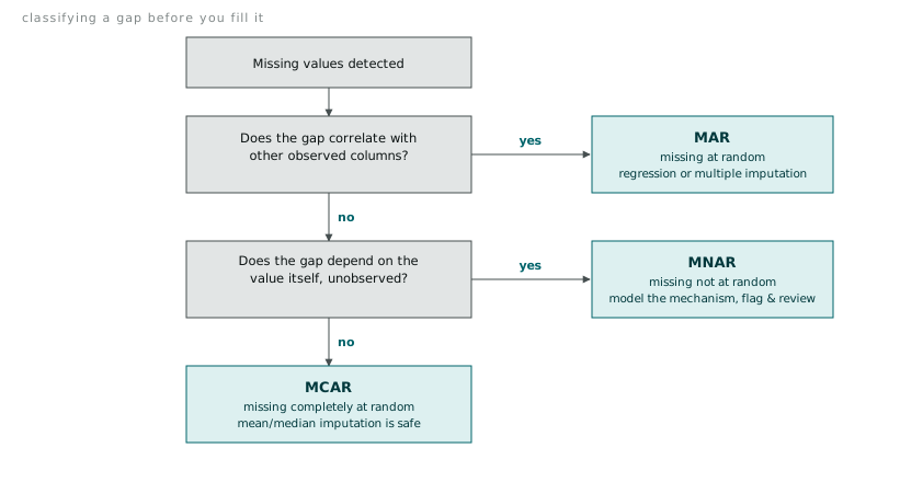
Once I know which mechanism I am dealing with, the imputation choice mostly falls out of it.
From simple imputation to something more careful
Mean and median imputation are the fastest options and the ones I still reach for first on an MCAR column with a low missing rate:
from sklearn.preprocessing import Imputer

imp = Imputer(missing_values='NaN', strategy='median', axis=0)
df['sensor_reading'] = imp.fit_transform(df[['sensor_reading']])
The problem is that mean imputation shrinks variance. Every imputed row lands on exactly the same value, so any downstream analysis that depends on the spread of the data, a standard deviation, a correlation, a regression coefficient, is quietly biased even when the missingness itself was MCAR and would not otherwise have caused a problem.
Regression imputation does better when the missingness is MAR. Train a model on the rows where the target is present, using the other columns as predictors, then use that model to fill the gaps:
from sklearn.linear_model import LinearRegression

train = df[df['income'].notnull()]
predict = df[df['income'].isnull()]

model = LinearRegression()
model.fit(train[['age', 'years_employed']], train['income'])

df.loc[df['income'].isnull(), 'income'] = model.predict(
    predict[['age', 'years_employed']]
)
This preserves the relationship between income and the predictors, which mean imputation destroys. It still understates uncertainty, because every imputed value is the model’s single best guess with no noise added back in. Multiple imputation addresses that by generating several plausible values per missing entry, drawn with some randomness, and pooling results across the resulting datasets. I know the theory, and I have read about the fancyimpute package doing MICE (multiple imputation by chained equations) in Python, but I have not put it into a production pipeline yet. For now, when the stakes are high enough to need it, I do the imputation in R with mice, which has had more time to mature.
Outliers, checked two different ways
Outlier detection splits the same way missing data does, along a single axis or across several at once.
Univariate detection looks at one column in isolation. The boxplot rule flags anything more than 1.5 times the interquartile range beyond the first or third quartile:
q1 = df['transaction_amount'].quantile(0.25)
q3 = df['transaction_amount'].quantile(0.75)
iqr = q3 - q1

lower_bound = q1 - 1.5 * iqr
upper_bound = q3 + 1.5 * iqr

outliers = df[(df['transaction_amount'] < lower_bound) |
              (df['transaction_amount'] > upper_bound)]
A z-score threshold does a similar job when the column is roughly normal: anything beyond 3 standard deviations from the mean is a candidate. I lean on the IQR rule more often, because it does not assume normality, and a handful of true outliers cannot drag the threshold around the way they can with a mean-based z-score.
Multivariate outliers are the ones that hide from both these checks. A customer whose age and income are each unremarkable on their own, a 22 year old earning $400,000, is not extreme in either column alone but is clearly an unusual combination. Mahalanobis distance catches this by measuring how far a point sits from the centre of the data once you account for the correlation between variables, rather than checking each column independently. I use it rarely, mostly because it is harder to explain to someone reading a report than “this value is more than three standard deviations out,” but on the fraud-adjacent work I have done it is the only method that catches the combinations that actually matter.
The rest of the taxonomy
Missing values and outliers get the most attention, but the taxonomy has three more categories worth naming.
Inconsistencies are values that are individually valid but disagree with each other in format or unit: a date column mixing DD/MM/YYYY and MM-DD-YYYY, a weight column mixing kilograms and pounds with no unit flag. Regex checks and unit audits catch these, similar to the extraction work I described in an earlier piece on regular expressions.
Duplicates range from exact row duplication, trivial to catch with a hash of the row, to fuzzy duplication where the same real-world entity appears under slightly different spellings or identifiers. That second kind deserves its own treatment, because the matching logic gets involved fast once you are merging more than one source.
Violations are values that break a rule the business already agreed on: a negative price, an end date before a start date, an age of 150. These are the easiest to catch and the easiest to ignore, because a violation does not look statistically unusual the way an outlier does. It just looks wrong to someone who knows the domain. I now write these rules down as explicit constraint checks that run before anything else, rather than trusting that a statistical outlier check will happen to catch them, because plenty of violations sit well inside a normal-looking range.
Treating “dirty data” as five distinct problems rather than one vague complaint is what turned my cleansing work from ad hoc poking into something I can plan for and estimate. I still cannot tell a stakeholder in advance exactly how many weeks a new dataset will take, but I can tell them which of the five categories I expect to be worst, and that has been enough to set reasonable expectations.