Implementing K-Means and Linear Regression on Spark Without MLlib

For two months, every model I trained on Spark went through MLlib. KMeans.train(), LinearRegressionWithSGD.train(), one line in, a fitted model out. It was the same shortcut I used to take with lm() in R, and it worked right up until I wanted to know why a k-means run over eight partitions gave slightly different final centroids to the same data run over one partition on my laptop. MLlib gave me no way to look at that difference from the inside. So I put it away for an afternoon and wrote k-means and linear regression as plain map and reduce jobs over RDDs, with no pyspark.mllib import anywhere in the file.

Map-reduce as a shape, not a Spark feature

Before touching Spark, I wrote the shape of the pattern in pure Python, on a list small enough to read by eye.

from functools import reduce

readings = [12.4, 15.1, 9.8, 22.3, 18.6, 14.2]

squared = list(map(lambda x: x ** 2, readings))
total = reduce(lambda a, b: a + b, squared)
mean_of_squares = total / len(readings)

map() applies the same function to every element independently, no element’s result depends on another’s. reduce() folds all those independent results down to one value by repeatedly combining pairs. Nothing here is distributed. The point was to separate the two ideas cleanly before adding a cluster underneath them, because once Spark’s RDD API is in the picture it is easy to treat map and reduceByKey as Spark-specific tools rather than a general pattern Spark happens to run in parallel.

The RDD mechanics that make this run across a cluster, lazy transformations, lineage, narrow versus wide dependencies, are the same ones I worked through with a word count a few weeks earlier in Spark RDD operations. A PySpark word count is the same shape as the Python snippet above, just handed to a SparkContext instead of a plain list:

lines = sc.textFile("readings.txt")
words = lines.flatMap(lambda line: line.split(" "))
pairs = words.map(lambda word: (word, 1))
counts = pairs.reduceByKey(lambda a, b: a + b)
counts.collect()

flatMap and map are the distributed version of my map() call above, one function applied independently per line. reduceByKey is the distributed reduce(), except it groups by key first and combines within each group, which is where the shuffle enters. Once that mapping was clear in my head, gradient descent stopped looking like a special case. It is the same shape, applied to rows of training data instead of words.

Gradient descent expressed as map and reduce

I had already derived the update rule for batch gradient descent by hand, working through the maths on eight rows in R in Deriving Gradient Descent by Hand. The rule itself does not change on Spark. What changes is how the gradient gets computed: instead of one process summing over every row, each partition sums over its own rows, and the driver combines the partial sums.

def compute_partial_gradient(partition):
    local_sum_w0 = 0.0
    local_sum_w1 = 0.0
    count = 0
    for x, y in partition:
        pred = w0.value + w1.value * x
        error = y - pred
        local_sum_w0 += error
        local_sum_w1 += error * x
        count += 1
    yield (local_sum_w0, local_sum_w1, count)

def train_linear_regression(data_rdd, iterations=200, alpha=0.01):
    w0_val, w1_val = 0.0, 0.0
    for i in range(iterations):
        w0_bc = sc.broadcast(w0_val)
        w1_bc = sc.broadcast(w1_val)
        globals()["w0"], globals()["w1"] = w0_bc, w1_bc

        partials = data_rdd.mapPartitions(compute_partial_gradient).collect()
        sum_w0 = sum(p[0] for p in partials)
        sum_w1 = sum(p[1] for p in partials)
        n = sum(p[2] for p in partials)

        grad_w0 = -2.0 / n * sum_w0
        grad_w1 = -2.0 / n * sum_w1
        w0_val -= alpha * grad_w0
        w1_val -= alpha * grad_w1

        w0_bc.unpersist()
        w1_bc.unpersist()
    return w0_val, w1_val

data_rdd holds (x, y) pairs, partitioned across the cluster the way Spark decided when the RDD was created. mapPartitions runs compute_partial_gradient once per partition rather than once per row, which matters because it lets each partition accumulate its own running sum in a plain Python loop instead of shipping every row’s contribution back individually. broadcast() sends the current weights out to every executor before the map step runs, so each partition computes its gradient against the same w0 and w1 the driver is currently holding, then the driver collect()s the partial sums and finishes the reduction itself with ordinary Python addition.

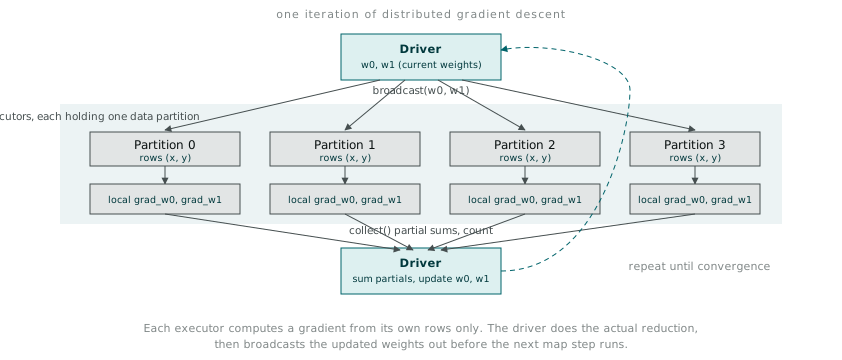
The first version I wrote called .reduce() directly on the RDD instead of collecting partials and summing in Python, and it worked, but it also meant a full RDD action and a fresh pass through the lineage on every single iteration, two hundred shuffles for two hundred iterations against genuinely small data. I switched to mapPartitions plus a Python-side sum on the collected results specifically because with two hundred iterations, the accumulated shuffle overhead of two hundred separate reduce actions dwarfed anything the toy dataset itself cost to process. On a dataset large enough to need Spark for real, the trade flips, and reduceByKey or treeReduce earns its keep. For anything smaller than that, an iterative distributed loop pays its shuffle tax once per iteration regardless of how little data sits behind it, which single-machine gradient descent never has to think about at all.

K-means as the same pattern, one level up

K-means fits the map-reduce shape almost exactly, because the two steps of Lloyd’s algorithm, assign points to the nearest centroid, then recompute each centroid as the mean of its assigned points, split cleanly into a map and a reduceByKey.

import math

def euclidean(a, b):
    return math.sqrt(sum((x - y) ** 2 for x, y in zip(a, b)))

def nearest_centroid(point, centroids):
    distances = [
        (i, euclidean(point, c)) for i, c in enumerate(centroids)
    ]
    return min(distances, key=lambda d: d[1])[0]

def assign_step(row, centroids_bc):
    cluster_id = nearest_centroid(row, centroids_bc.value)
    return (cluster_id, (row, 1))

def sum_points(a, b):
    point_a, count_a = a
    point_b, count_b = b
    summed = [p1 + p2 for p1, p2 in zip(point_a, point_b)]
    return (summed, count_a + count_b)

def kmeans(data_rdd, k, max_iterations=50, tolerance=1e-4):
    centroids = data_rdd.takeSample(False, k, seed=42)

    for iteration in range(max_iterations):
        centroids_bc = sc.broadcast(centroids)

        assigned = data_rdd.map(lambda row: assign_step(row, centroids_bc))
        summed_by_cluster = assigned.reduceByKey(sum_points)

        new_centroids = summed_by_cluster.map(
            lambda kv: (kv[0], [d / kv[1][1] for d in kv[1][0]])
        ).collect()

        new_lookup = dict(new_centroids)
        max_shift = max(
            euclidean(centroids[i], new_lookup[i]) for i in new_lookup
        )

        centroids = [new_lookup[i] for i in sorted(new_lookup)]
        centroids_bc.unpersist()

        if max_shift < tolerance:
            break

    return centroids

assign_step is the map, run once per point, entirely independent across points, exactly the property that made word count’s flatMap step embarrassingly parallel. reduceByKey(sum_points) is where the actual reduction happens, combining every point assigned to cluster i, wherever it lives across the cluster’s partitions, into one running sum and count. Dividing that sum by its count gives the new centroid mean, no different in principle from the mean I would compute with df.groupby("cluster").mean() on a single machine, just computed via a shuffle instead of an in-memory groupby.

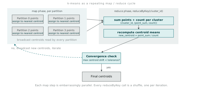
The convergence check matters more here than it did for gradient descent, because k-means genuinely can oscillate between two assignments on data with ambiguous cluster boundaries, points sitting almost exactly between two centroids that get reassigned back and forth each pass without the centroids themselves ever settling. max_shift < tolerance catches the case where centroids stop moving meaningfully, but it does nothing about points still flipping cluster membership with no real effect on the centroid position. I found that out by running max_iterations=50 against synthetic data with two centroids I deliberately placed close together, watching the loop use every iteration it was allowed without the max_shift ever dropping below tolerance, because a handful of boundary points kept swapping sides each pass, nudging each centroid a fraction each time, forever.

What changes when the reduce step costs a shuffle

The version of these algorithms I would write for a single machine, sklearn.cluster.KMeans or a plain NumPy gradient descent loop, treats every iteration as cheap. Loop count barely matters because each pass is a few array operations sitting in memory. On Spark, every iteration through reduceByKey is a stage boundary, a shuffle, data written out, redistributed by key across the network, read back before the next map step can start. That cost does not show up anywhere in the algorithm’s maths. It shows up in wall-clock time, and it means an implementation choice that looks equivalent to a single-machine version, running to convergence with a tight tolerance and a generous iteration cap, can be the difference between a job that finishes in under a minute and one that is still shuffling twenty minutes later over data that would fit in memory on a decent laptop.

That is the trade MLlib is making underneath its one-line calls: fewer, better-batched reduce operations, careful choices about when to cache an RDD across iterations rather than recomputing it, decisions about partition count tuned to avoid both an underused cluster and a shuffle with too many small partitions. None of that is visible from KMeans.train(). It is exactly what shows up once you write the loop yourself and watch the Spark UI fill up with one stage per iteration, each one waiting on the slowest partition in the reduce step before the next map can begin.