I spent the first two weeks with Spark writing DataFrame code and getting away with it. df.groupBy("word").count() reads almost like SQL, the Catalyst optimiser does something clever underneath, and results come back. It worked well enough that I did not ask what was underneath it until a collect() on a modest join hung for four minutes and I had no idea why. The DataFrame API had given me no vocabulary to reason about what was slow. RDDs gave me that vocabulary back.
An RDD, a Resilient Distributed Dataset, is Spark’s original data structure: an immutable collection of objects split across partitions on a cluster, computed through a chain of transformations Spark remembers rather than executes on the spot. Every DataFrame is still an RDD underneath, wrapped in schema information and an optimiser. Once I understood how RDDs actually run, DataFrame behaviour stopped feeling mysterious.
Getting a shell running and a file loaded
I did this in spark-shell against Spark 2.1.0 with Scala 2.11.6, using the README that ships with every Spark install as a source file, because it is small, always there, and nobody has to explain what it contains.
scala> val lines = sc.textFile("README.md")
lines: org.apache.spark.rdd.RDD[String] = README.md MapPartitionsRDD[1] at textFile at <console>:24
sc is the SparkContext, the shell hands you one automatically. textFile reads the file into an RDD of lines, one string per line, split across however many partitions Spark decided to use based on the file’s block size. Nothing has been read from disk yet. textFile is a transformation, and Spark transformations do not run until something forces them to.
Transformations build a plan, they do not run it
This surprised me the first time I hit it. I ran the line above expecting Spark to read the file, and instead it returned instantly with a description of an RDD, not its contents.
scala> val words = lines.flatMap(line => line.split(" "))
words: org.apache.spark.rdd.RDD[String] = MapPartitionsRDD[2] at flatMap at <console>:25

scala> val pairs = words.map(word => (word, 1))
pairs: org.apache.spark.rdd.RDD[(String, Int)] = MapPartitionsRDD[3] at map at <console>:26

scala> val counts = pairs.reduceByKey(_ + _)
counts: org.apache.spark.rdd.RDD[(String, Int)] = ShuffledRDD[4] at reduceByKey at <console>:27
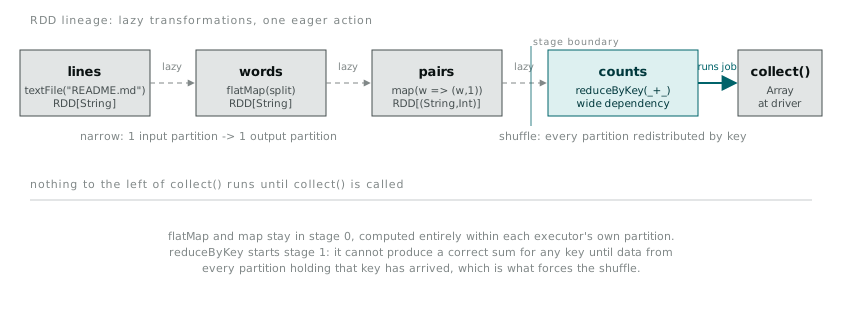
Four RDDs now exist in the shell’s variable bindings, lines, words, pairs, counts, and none of them holds any actual data yet. Spark has instead built a lineage graph, a record of how to produce each RDD from its parent if asked. flatMap splits each line into words and flattens the resulting lists into one RDD of words. map turns each word into a (word, 1) pair. reduceByKey groups pairs by key and sums the values, which is where a shuffle first enters the picture, more on that below.
This laziness is not an implementation quirk, it is the whole point. Spark can look at the full chain of transformations before running any of it and decide how to execute the plan efficiently, the same way a query planner looks at a full SQL statement rather than running each clause the moment it is typed.
Actions are what actually trigger a job
Nothing computed until I called an action, a method that returns a concrete result to the driver rather than another RDD.
scala> val results = counts.collect()
results: Array[(String, Int)] = Array((package,1), (this,1), (Version,1), ...)

scala> counts.count()
res1: Long = 546

scala> counts.take(5)
res2: Array[(String, Int)] = Array((package,1), (this,1), (Version,1), (Because,1), (Python,2))
Calling collect() is the moment Spark walks the lineage graph backwards from counts, works out which partitions need to be read, and schedules the actual work. count() and take(5) are both actions too, and each one triggers a fresh run of the same lineage unless something has been cached, which brings up the next problem I ran into.
Why caching matters, learned the expensive way
I called counts.count() immediately after counts.collect() in the same session, assuming the second call would be fast since Spark had “just done this.” It was not fast. Both calls re-read README.md, re-ran flatMap, re-ran map, and re-ran reduceByKey, because an RDD’s lineage describes how to build it, not a cache of what building it produced last time. Nothing is stored unless told to be.
scala> counts.cache()
res3: counts.type = ShuffledRDD[4] at reduceByKey at <console>:27

scala> counts.count()  // first call after cache(), still runs the full job, but stores the result
res4: Long = 546

scala> counts.count()  // second call, reads from cached partitions instead
res5: Long = 546
cache() is shorthand for persist(StorageLevel.MEMORY_ONLY). It does not force computation itself, it only marks the RDD as one to keep in memory once it is computed. The first action after cache() still pays the full cost of running the lineage. Every action after that reads the stored partitions instead of recomputing them. For a word count run once, caching buys nothing. For an RDD reused across several downstream actions, which is the common case once real analysis starts, skipping caching means paying for the same shuffle and the same file read every single time.
Narrow versus wide, and why reduceByKey is the expensive step
Not every transformation costs the same, and the distinction comes down to whether an output partition needs data from exactly one input partition or from all of them.
flatMap and map are narrow dependencies. Each output partition depends on exactly one input partition, so Spark can run them entirely inside the executor that already holds the data, no network traffic involved. reduceByKey, on the other hand, is a wide dependency. To sum the count for the word “Spark”, Spark needs every occurrence of “Spark” in one place, and those occurrences can be scattered across every partition in the cluster. That forces a shuffle, data gets written out, redistributed across the network by key, and read back in on the other side before the reduce step can run.
This is the same operation I built by hand with Python’s multiprocessing.Pool a few months back, hash-partitioning two files by key before a parallel join, in Implementing Parallel Search, Join, and Sort From Scratch. reduceByKey does exactly that repartition step, except Spark decides the partition count, handles the network transfer, and spills to disk if a partition does not fit in memory, none of which my hand-rolled version did.
How a job actually runs on a cluster
Calling collect() sets off a chain that starts at the driver program, the process running my shell session, and works outward.
The driver asks the cluster manager, which was YARN on the machine I was using, for executor processes. Each executor gets assigned a set of partitions to hold and runs tasks against them, one task per partition per stage. Spark splits the overall job into stages at shuffle boundaries, because everything before a shuffle can run independently per partition, and everything after it needs the shuffle to finish first. In the word count lineage, textFile, flatMap, and map all run inside a single stage, since none of them need data from another partition. reduceByKey starts a new stage, because its input is the shuffled output of the first stage, not the raw partitions textFile created.
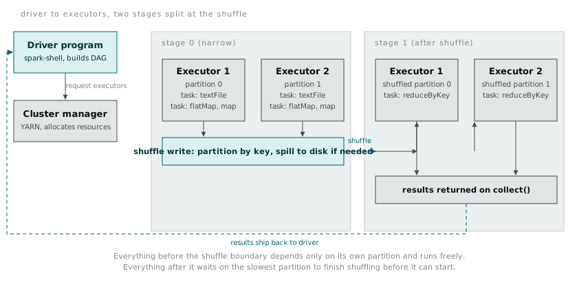
That four-minute hang I mentioned at the start turned out to be a groupBy on a DataFrame with a badly skewed key, one value present in roughly forty percent of the rows, which meant one shuffle partition held forty percent of the data and one executor sat there alone doing forty percent of the work while every other executor finished in seconds. The DataFrame plan explorer in the Spark UI showed a stage with wildly uneven task durations, but understanding what “stage” and “shuffle” actually meant, at the RDD level, is what let me read that UI at all. I split the skewed key into a compound key with some added salt, spread the load, and the same job finished in twenty seconds.
What this bought me
None of this changes how I write day-to-day Spark code. DataFrames stay the default, the optimiser earns its keep, and I am not about to hand-write flatMap chains for production jobs. What changed is what happens when a job is slow or wrong. “It is stuck in a shuffle” used to be something I repeated because someone else said it. Now it means something specific: a wide dependency somewhere in the plan is waiting on every partition to finish before it can start reducing, and if one of those partitions is far bigger than the rest, the whole stage waits on it. That is not a Spark mystery. It is a partitioning problem, and partitioning problems have partitioning solutions.