When I worked through PCA, k-means, and hierarchical clustering last year, the thing that stuck with me longest about PCA was how mechanically simple it is underneath. It is one matrix multiplication, projecting your data onto whichever directions capture the most variance, found via eigendecomposition of the covariance matrix. That simplicity is also its ceiling. PCA can only find linear structure, straight lines and flat planes through the data, because a matrix multiplication is a linear operation no matter how you dress it up. If the true structure in your data curves, sits on some bent manifold rather than a flat subspace, PCA will still give you an answer, and that answer will still be wrong in a way no amount of adding more components fixes.
An autoencoder is what happens when you ask a neural network to do the same compression job PCA does, but let it use nonlinear activation functions to get there. Having just spent two months getting comfortable with Keras for basic classification, building an autoencoder felt like a natural next experiment, mostly because it needs no labels at all, which connects it back to the unsupervised side of things I had mostly left behind once I moved on to neural networks.
The architecture: a bottleneck in the middle
An autoencoder has a distinctive shape. It is symmetric, narrowing down to a bottleneck in the middle and then widening back out to the original size, and it is trained to reproduce its own input as its output.
from keras.models import Model
from keras.layers import Input, Dense

input_img = Input(shape=(784,))
encoded = Dense(128, activation='relu')(input_img)
encoded = Dense(64, activation='relu')(encoded)
encoded = Dense(32, activation='relu')(encoded)
bottleneck = Dense(16, activation='relu')(encoded)

decoded = Dense(32, activation='relu')(bottleneck)
decoded = Dense(64, activation='relu')(decoded)
decoded = Dense(128, activation='relu')(decoded)
decoded = Dense(784, activation='sigmoid')(decoded)

autoencoder = Model(input_img, decoded)
I used the functional API rather than Sequential here, mostly out of habit from wanting to keep the encoder addressable as its own model later, though a plain Sequential stack would work just as well for training the autoencoder itself. The first half, from the 784 dimensional input down to the 16 dimensional bottleneck, is the encoder. It squeezes the image down through progressively narrower layers, 128, then 64, then 32, then 16, forcing the network to decide what information is worth keeping at each stage. The second half, mirroring those widths back up, 32, 64, 128, and finally 784 again, is the decoder, trying to reconstruct the original image from nothing but that 16 dimensional summary.
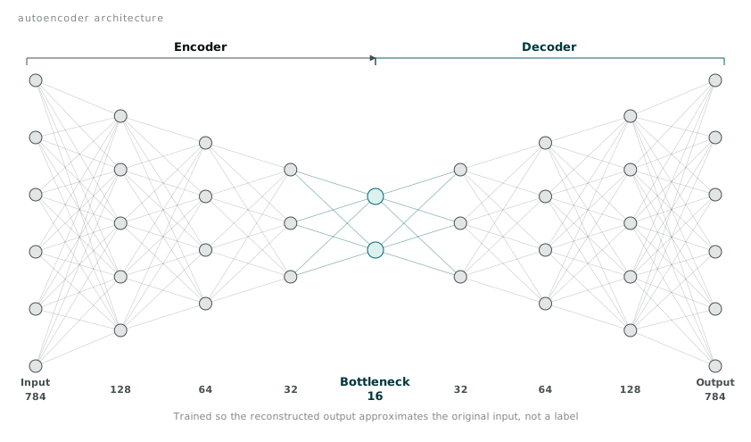
The 16 dimensional bottleneck is the whole point. Every one of the 784 pixel values in the reconstructed output has to be derived from just 16 numbers, so those 16 numbers had better capture whatever matters about the digit, its shape, its stroke width, roughly which class it belongs to, because nothing else survives the trip through the middle. That is a much harder constraint than PCA’s version of the same idea, and the nonlinear activations at every layer are what let the network satisfy it in ways a straight linear projection cannot.
Training without labels
The loss function is where autoencoders depart most obviously from the classification work I had been doing. There is no y_train in the usual sense, no separate label array at all. The target the network is trying to match is its own input.
autoencoder.compile(optimizer='adam', loss='binary_crossentropy')

autoencoder.fit(
    x_train, x_train,
    epochs=50,
    batch_size=256,
    validation_data=(x_test, x_test)
)
Passing x_train as both the input and the target the first time felt like a typo waiting to happen, and I did in fact stare at it for a moment wondering if I had made an error before remembering that this is exactly the point. binary_crossentropy as the loss works here because the pixel values, scaled to between 0 and 1, and the sigmoid output activation both behave like probabilities pixel by pixel, even though this is not really a classification problem in the usual sense. Mean squared error is the more common alternative and I tried both, finding binary cross entropy gave marginally sharper reconstructions on this dataset, though I would not read too much into one comparison on one dataset.
After training, checking reconstruction quality meant running test images through the full network and comparing them against the originals by eye.
import matplotlib.pyplot as plt

reconstructed = autoencoder.predict(x_test)

n = 10
plt.figure(figsize=(20, 4))
for i in range(n):
    ax = plt.subplot(2, n, i + 1)
    plt.imshow(x_test[i].reshape(28, 28), cmap='gray')
    ax = plt.subplot(2, n, i + 1 + n)
    plt.imshow(reconstructed[i].reshape(28, 28), cmap='gray')
plt.show()
The reconstructions are recognisably the same digits, slightly blurred, edges softened, occasionally a 4 that looks like it is second-guessing whether it wants to be a 9. That blur is the visible cost of compressing 784 numbers down to 16 and back, and it is a genuinely useful way to see the information loss happening rather than just reading it off as a loss number in a training log.
Pulling the encoder out on its own
Once the whole autoencoder is trained, the encoder half is useful entirely on its own, as a dimensionality reduction tool that happens to have learned nonlinear structure instead of linear structure.
encoder = Model(input_img, bottleneck)
encoded_imgs = encoder.predict(x_test)
print(encoded_imgs.shape)  # (10000, 16)
That gives every test image a 16 dimensional representation instead of 784, learned entirely without ever being told which digit was which. I ran a quick 2D visualisation using just two of the encoded dimensions plotted against each other, coloured by the true digit label purely for checking the result rather than for training, and digits of the same class visibly clustered together even though nothing about class membership went into training the autoencoder. That was the moment the unsupervised angle clicked properly. The network found structure that correlates strongly with digit identity purely by trying to compress and reconstruct pixels.
Where PCA and autoencoders actually differ
Putting this side by side with PCA made the practical difference between linear and nonlinear compression concrete rather than abstract. Imagine data sitting along a curved arc in a 2D plane rather than a straight line. PCA can only fit a straight line through it, its best single component, and every point gets projected onto that line regardless of where along the curve it actually sits, which means points from quite different parts of the arc can end up mapped to nearly the same value. An autoencoder with nonlinear activations can, in principle, learn to follow the curve itself, unrolling it into a straight coordinate rather than flattening it onto one.
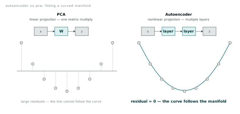
That extra flexibility is not automatically an advantage. PCA’s solution is deterministic, exact for the objective it optimises, and takes seconds to compute even on fairly large datasets. The autoencoder’s solution depends on architecture choices I mostly guessed at, layer widths, how many layers, which activation functions, and on a training process that can land in different local minima depending on the random initialisation of the weights, meaning two runs on the same data will not produce identical encoders. For data that genuinely is close to linear, PCA will find that structure just as well with a fraction of the effort and none of the uncertainty. The autoencoder earns its complexity specifically when the underlying structure curves in ways a flat subspace cannot follow, and knowing which situation you are in ahead of time is not always obvious. I suspect that judgement only comes from running both and comparing, which is roughly how I ended up understanding the difference in the first place.